The Kanban system is a method of using cards as visual signals for triggering or controlling the flow of materials or parts during the production process. It synchronizes the work processes within your own organization as well as those that involve your outside suppliers. The Japanese word Kanban which is translated as “signboard”, has been seen as the substitute works of demand scheduling. In the late 1940s and early 1950s, Taiichi Onho developed Kanban to control production between processes and to implement Just in Time manufacturing at Toyota manufacturing plants. And the strategy of Kanban became one of the pillars of Toyota’s successful implementation of JIT manufacturing. However, these Kanban ideas hadn’t been accepted until the global economic recession blown the world. Under the global recession, people saw that Kanban could minimize the work in process (WIP) between processes and reduce the cost associated with holding inventory as well. The modern Kanban has been developed a lot comparing with the Japanese Kanban, which is seen as a software tool of Lean.
Definition of Kanban
From different stages of Kanban development and the functions, Kanban has different definition. Some are more close to what is used in Toyota, some are more developed as a component of Lean. Two definitions will be showed below to form an overall understanding of Kanban.
Definition one
Kanban is defined as demand scheduling. In processed controlled by Kanbans, the operators produce products based on actual usage rather than forecasted usage. The Kanban schedule replaces the traditional weekly or daily production schedule. This schedule is replaced with visual signals and predetermined decision rules that allow the production operators to schedule the line. What Kanban replace is:
The daily scheduling activities necessary to operate the production process;
The need for production planner and supervisors to continuously monitor schedule status to determine the next item to run and when to change over. (John M.Gross, 2003)
In this case, it frees the materials planners, schedulers and supervisors to manager exception and to improve the process. Finally, it also places control at the value-added and empowers the operators to control the line.
Definition two
Kanban is a lean agile system that can be used to enhance any software development life-cycle including Scrum, XP, Waterfall, PSP/TSP and other methods. Its goal is the efficient delivery of value. (Linden-Reed, 2010)
Kanban promotes the lean concept of flow to continuously and predictably deliver value;
The work and the workflow is made visible to make activities and issue obvious;
Kanban limits WIP to promote quality, focus and finishing.
Comparing with the first definition, the second one is more abstract. It is defined by what functions it could deliver.
Need for Kanban system
In the Kanban system, a card (called a Kanban) controls the movement of materials and parts between production processes. A kanban moves with the same materials all the way down the production line. When a process needs more parts or materials, it sends the corresponding Kanban to the supplier; the card acts as the work order. A kanban card contains the following data:
What to produce
How to produce it
When to produce it
How much to produce
How to transport it
Where to store it
In an ideal world, demand for products would be constant. Organizations could always operate at maximum efficiency, producing exactly what was needed—no more, no less. But for most companies, the amount of work that must be done varies by the day, week, or month. An organization must have enough capacity so that there are enough people, machines, and materials available to produce what is needed at times of peak demand. But when there is a smaller amount of work to be done, one of two things can happen: 1) Underutilization of people, machines, or materials or 2) overproduction. With the kanban system, workers are cross-trained to be knowledgeable about various machines and work processes so that they can work on different manufacturing tasks as needed. This prevents under utilization. Kanban systems also prevent overproduction, which is the single largest source of waste in most manufacturing organizations. When you use the kanban system correctly, no overproduction will occur. The kanban system also gives your organization the following positive results:
All employees always know their production priorities.
Employees’ production directions are based on the current conditions in your workplace. Employees are empowered to perform work when and where it is needed. They do not need to wait to be assigned a work task.
Unnecessary paperwork is eliminated.
Skill levels among your employees are increased.
Framework
Mass customization
Mass customization was initiated in 1987 by Stan Davis. The concept is defined by David as: “Mass customization is the ability to quickly and efficiently build-to-order customized products.” Practitioners of mass customization share the goal of developing, producing, marketing, and delivering affordable goods and services with enough variety and customization that nearly everyone finds exactly what they what. Mass customization is a new form of competition that has arisen in the global market place. As Pine summaries, there are three main forms to face this challenge: Japan Inc., flexible specialization communities, and dynamic extended enterprises. Each form was simply trying to find its way to competitive advantage in a world increasingly characterized by a high degree of market turbulence. To summaries the new competitions, there are positive effects of mass customization on different functions in a firm, e.g. the production function, R&D function, marketing function, and financial function. Here list the positive effects on production function.
Positive Effects
Low overhead and bureaucracy
Optimum quality
Elimination of waste
Continual process improvement
Low inventory carrying costs
High labor productivity
Integration of thinking and doing
High utilization of and investment in worker skills
Sense of community
Low total costs
High production flexibility
Greater variety at lower costs
The focus of the manufacturing production function of the new competition is on total process efficiency. Process efficiency includes both productive and unproductive time. Unproductive time is the time materials spend in inventory or other non-operational activities such as handling, moving, inspecting, reworking, recoding, batching, chasing, counting, and repacking…. (Michael) According to the above table, the mass customization has potential to do changes on these aspects of production. When facing the new frontier of mass customization, there are proper strategies to response. There are three basic ways to do this: incrementally over time, more quickly via business transformation, or by creating a new business firmly planted in the new territory.
Strategic Response
When Appropriate
Move Incrementally
Market turbulence low and not increasing dramatically
Competitors not transforming for Mass Customization
Middle-and lower-level managers and employees who want to change but cannot affect the business as a whole
Transform the Business
Dramatic increase in market turbulence
Competitors already shifting to Mass customization
Only if instigated or fully supported by top management
Create a New Business
Businesses based on new, flexible technologies
New ventures in large corporations
Most any new business
Lean Manufacturing
Lean manufacturing is a generic process management philosophy derived mostly from the Toyota Production System (TPS). Lean manufacturing or lean production is often simply known as “Lean‟. The core idea of lean is to maximize customer value while minimizing waste. Lean means creating more value for customers with fewer resources. A lean organization understands customer value and focuses its key processes to continuously increase it. The ultimate goal is to provide perfect value to the customer through a perfect value creation process that has zero waste. To achieve this, lean thinking changes the focus of management from optimizing separate technologies, assets, and vertical departments to optimizing the flow of products through entire value streams that flow horizontally across technologies, assets, and departments to customers.
Lean principles
There are five main principles of lean manufacturing: value specification, value stream, flow, pull and perfection.
Specify value
Overproduction
Waiting
Unnecessary transport
Over processing
Excess inventory
Unnecessary movement
Defects
Unused employee creativity
The main non-value-adding waste is overproduction, because it could generate other wastes. However, making flow does simply mean to eliminate waste one by one. It needs much preparation work and a holistic vision which guides a strategy towards flow.
Identify the value stream
The value stream is the set of all the specific actions required to bring a specific product through the three critical management tasks of any business. (Womack and Jones, 1996) identifying the entire value stream for each product is the next step in lean thinking. Lean thinking must go beyond the firm to look at the whole. Creating lean enterprises requires a new way to think about firm-to-firm relations, some simple principles for regulating behavior between firms, and transparency regarding all the steps taken along the value stream so each participant can verify that the other firms are behaving in accord with the agreed principles.
Flow
The third principle is Flow. Once value has been specified, the value stream for a specific product fully mapped and obvious wastes eliminated, it is time to make the remaining, value-creating steps flow. However the traditional “functions” and “departments” concepts always block producers realizing real flow. The performing tasks in batches are always thought as best. The batches and queues are common used by most manufacturers blinding other common senses. The lean thinking is to redefine the work of functions, departments, and firms so they can make a positive contribution to value creation and to speak to the real needs of employees at every point along the stream so it is actually in their interest to make value flow. There are three steps to make value flow. The first step, once value is defined and the entire value stream is identified, is to focus on the actual object and never let it out of sight from start to finishing. The second step is to ignore the traditional boundaries of jobs, careers, functions and firms to form a lean enterprise removing all impediments to the continuous flow of specific product or product family. The third step is to rethink specific work and tools to eliminate backflows, scrap, and stoppages of all sorts so that the design, order and production of the specific product can proceed continuously. There are also some practical techniques to prepare for flow:
Level out workloads and pace production by Takt time/pitch time;
Standardizing work and operating procedures;
Total productive maintenance;
Visualize management;
Reduce changeover;
Avoid monuments and think small
Pull
The subjective of pull is customer orders. Let the customer pull the product rather than pushing products onto the customer. It means short-term response to the rate of customer demand without overproduction. There are two levels which express the meaning of pull. On the macro level, the production process should be triggered by customer demand signals. The trigger point is expected to be pushed further and further upstream. On the micro level, there is responding to pull signals from an internal customer that may be the next process step I the case of Kanban or an important stage in the case of Drum/Buffer.
Perfection
The final one is Perfection. Perfection means producing exactly what customers want, exactly when without delay, at a competitive price and with minimum waste. The real benchmark is zero waste, not what competitors do.
The five powerful ideas in the lean tool kit needed to convert firms and value streams from a meandering morass of muda to fast-flowing value, defined and then pulled by the customer. And it reveals the inherent thinking to pursue perfection. The techniques themselves and the philosophy are inherently egalitarian and open. Transparency in everything is a key principle.
Just-In-Time
Just-in-time (JIT) is developed by Taichi Ohno and his fellow workers at Toyota, one of the pillars of TPS. It means to supply to each process what is needed when it is needed and in the quantity it is needed. The main objective of JIT manufacturing is to reduce manufacturing lead times which is primarily achieved by drastic reductions in work-in-process (WIP). The result is a smooth, uninterrupted flow of small lots of products throughout production. These stock reductions will be accompanied by sufficiently great improvements in quality and production to result in unheard-of cost reductions. There are three main kind of stockholding: incoming material, work-in-process and finished goods. JIT aims to reduce each of them through a holistic principle. In the following text, the principle will be illustrated through each stockholding.
Incoming material
The incoming material control is always relates to a firm´s purchasing policy and its suppliers. In reality, the incoming material is unreliable or unpredictable. The excessive stocks and stock out of incoming material are always happen. What firm should do is to involve its suppliers into their own manufacturing instead of tell them what to do.
Work-in-process
In the factory buffer stocks exist everywhere in several forms. WIP is always been a key industrial measure. The total value forms part of the balance sheet, and industrial managers are under intense pressure to keep the figures as low as possible. However, there are many causes contribute to a high WIP. The causes include:
Production scheduling
Machine capability
Operator capability
Product mix
Product modification
Changing product priorities
Cross-functioned organization
Machine breakdown
In order to achieve low WIP, JIT provides principles to deal with the above obstacles. There are some main principles mentioned as following:
Level out the workload and pace production.
JIT techniques work to level production, spreading production evenly over time to make a smooth flow between processes. Varying the mix of products produced on a single line, sometimes, provides an effective means for producing the desired production mix in a smooth manner.
Pull production.
With pull system, Kanban is always used. To meet JIT objectives, the process relies on signals or Kanban between different points in the process, which tell production when to make the next part. Implemented correctly, JIT can improve a manufacturing organization’s return on investment, quality, and efficiency. Its effective application cannot be independent of other key components of a lean manufacturing system.
Finished goods
In an idea JIT production operating the pull system, there will be no finished goods in stock. Even though the stockholdings would be illustrated separately, JIT should be designed as a whole principle to reduce the stockholdings on a holistic level. To summarize, JIT is pulling work forward from one process to the next “just-in-time”. One benefit of manufacturing JIT is reducing work-in-process inventory, and thus working capital. An even greater benefit is reducing production cycle times, since materials spend less time sitting in queues waiting to be processed. However, the greatest benefit of manufacturing JIT is forcing reduction in flow variation, thus contributing to continuous, ongoing improvement.
Selecting the physical signaling for the Kanban
When people think of Kanban, most of them will think of Kanban cards. Actually, there are different types of physical Kanbans could be applied in production system. Each company could definitely do some innovation on their own physical Kanban regarding of their unique production systems.
Kanban cards
Kanban cards are essentially pieces of paper which travel with the production item and identify the part number and amount in the container. Kanban cards serve as both a transaction and communication device. The following figure shows a Kanban card used between processes.
Kanbans using cards signal often follow the routines below:
A card is placed with the completed production container;
The container with its Kanban card is then moved into a staging area to wait for use;
When the container is moved to production work center for use, the Kanban card is pulled from the container to signal consumption.
The Kanban card is then placed in a cardholder, or Kanban post, to await transit back to the production line;
When the Kanban card returns to the production line, it is placed in a cardholder that has been set up to provide a visual signal for operation of the line;
The Kanban card sits in the cardholder waiting to be attached to a completed production container.
The Kanban cards illustrated here mainly concern the concept used in Toyota production system. Individual company could do any verification regarding of its own condition. However, this Kanban card is more useful in assembly line than other type of production line.
Kanban boards
Kanban boards simply use magnets, plastic chips, colored washers, etc. as signals. The objects represent the items in inventory- backlog, in-process inventory. It helps to visualize the workflow, limit WIP and measure the lead time. There is a sample of Kanban board. Each firm could develop the column detail according to its own production condition.
The two columns stands side shows the product backlog and finished products. And the column in between illustrate the sequence processes. The stick notes are updated by operators going from backlog to finished products. To determine what gets produced next, operators just look at the board and follow its rules. Kanban boards work best when two conditions exist in the relationship of inventory storage and the production process:
The board can be positioned in the path of the flow of all the material to the customer;
The board can be positioned so that the production process can see it and follow the visual signals.
Two-card Kanban
Two-card Kanban is typically used for large items where flow racks are not utilized. It is a combination system of the Kanban board and the Kanban card racks. It works like this:
When product is produced or received from a vendor, two cards are pulled from a Kanban card rack and filled out: one Kanban card goes with the container; the second Kanban card goes into a special FIFO box.
Whenever a container of this product is needed, a material handler goes to the FIFO box and pulls out the bottom card.
The material handler then goes to the location written on the card and pulls this product for the production operation.
The material hander then takes both cards and places them in the Kanban card racks, which show the schedule signals for production or record.
This system allows pallet size items to flow while managing product rotation. It works especially well when used for floor stacked items.
Look-see
Look-see is a Kanban signal that behavior relying on the sensor of people` eyes. It includes visual signals such as floor marking that shows when to replenish the item. The basic rule with a look-see signal is that when yellow signal signs, then it is time to replenish the item. The red, or danger, signal is also integrated into this scheme. Look-see signals greatly aid in the implementation of the Kanban supermarkets.
Little´s Law
Little´ s law is firstly proved by John little in 1961. In queuing theory, it says: “The average number of customers in a stable system (over some time interval) is equal to their average arrival rate, multiplied by their average time in the system. Although it looks intuitively reasonable, it’s a quite remarkable result. “ The strength of Little´s law is the fact that is makes no assumption about the probability distribution of arrival rate or service rate, or if they make a first-in-first-out queues, or some other order in which they are served. The only pre-condition or requirement for Little´s Law to hold is that it must be applied to a stable or a steady state system. Little´s law one thing that constant and true in manufacturing field. In manufacturing field, little´s law could be expressed as: cycle time in time unit is equal to amount of work in process in units, divided by the output in units during this time unit. This is to say that if the total units throughout the work areas and the output per time unit are constant, the cycle time could be easily got. It is also true that if the WIP remains constant and the output is decreased, the cycle time will go up. And if the Takt is constant, when reducing the WIP, the cycle time would be reduced. If manufacturing could maintain close control over the cycle time of its product, from the input point till the completely release point, it could predict to customers what they expect in terms of delivery. If the process were completely under control, there could be no problem in guaranteeing delivery date. The customer satisfactory could be increased. In realistic manufacturing, manufacturing processes are mostly hard to predict. Problems occur everywhere, e.g. operator absence, machine breaking down, vendor problems etc. If the input is the same, and the output goes down, WIP will most definitely build up at the bottleneck. It is know that the bottleneck could change the pace until the problems are fixed. Little´s law tells that how much it could raise or lower the output. Once product is launched in shop floor, it is crucial to do everything to keep it moving. If the products are stuck somewhere, it is better to slow or stop launching new products in the production system. According to little´s law, if a production system is expected to increase its output, the way is not to increase the input amount when its output levels can`t be reached. The best way is to find the bottleneck and increase its output. Little´s law suggests that don‟t operate on the edge of capability or accept orders that challenge the edge of production capacity. If it does, there is a risk to prolong the delivery dates. Little´s law backs up the Flow theory in manufacturing field. Idealistically, if it is one-piece-flow, the output is much easy to predict and the cycle time would be limited to its extreme.
Determine rules of Kanban
Before developing rules for Kanban implementation, it is essential to make materials and physical Kansans to move in a continuous flow. This is to determine how material and physical Kanban move through the production process, and how the move Kanban go back to production process when they are released.
The rules for developing the Kanban are its driving force. The rules are the guidance to allow the operation unit staffs to control the production schedule. The rules should include:
The part numbers covered by the Kanban;
How the design works-how the cards, magnets, etc., move
The meaning of the scheduling signals and how to interpret them;
Any scheduling rules of thumb;
The preferred production sequence
Who to go to and what the “helpers” should do when contacted;
Any special quality or documentation requirements.
When creating rules, one thing should be in head all the time: the rules are to communicate how to run the Kanban and to allow the process operator to schedule the line. The only way the production operators can take over scheduling the line is by the rules providing clear direction and scheduling guidance. When drafting the scheduling rules make them easy and unambiguous to follow. Think through possible misconceptions and correct them so they will not occur. Spell out what signals a normal changeover. Spell out what signals emergency changeover. Seek feedback to make sure that everyone else is as clear about how to interpret the signals as asked. Additionally, the scheduling rules should contain clear-cut decision rules. The decision rules should help the production operators make consistent production scheduling decision based on the stated priorities. The rules should provide rate information, if applicable, to allow the operator to develop production expectation. The decision rules should contain instructions on when and whom to call for help. Also the rules should include all the “everyone knows this” items that everyone seems to forget from time to time.
Create a visual management plan
The visual management plan will explain the Kanban to everyone and visually instruct everyone how the Kanban operates. The basic goal of visual aids should be to answer the questions that pop up on a daily basis: where do I get this from, where do I move that, which color buggy contains which part, is there a color scheme, do we have any more of this part? To make the visual aids colorful and easy to read. There are some useful tips :
Keep the colors consistent with existing color schemes;
Avoid red-typically associated with safety or quality;
Avoid yellow-typically associated with safety;
Use large print for hanging signs and wall signs;
Avoid excessive words on signs-people don‟t read signs, they glance at them.
After the above three steps: Selecting the physical signaling for the Kanban; determine rules of Kanban; create a visual management plan. The Kanban design process could be finished.
Principles for Kanban design/ implementation
This part is to summarize the above Kanban implementing details and provide a general guidance. Here is a minimal way to implement Kanban:
Preparation stage:
Review entire workflow. Look at the end-to-end process from initial concept forward through release. Analyze for any excessive time pockets. Remember to look at handoff times.
Address bottlenecks. If bottlenecks are found, including upstream of the engineering phase, work to break them down and deliver their value in small increments.
Switch from iterations to SLA(Service level Agreement). Forget about iteration time-boxes because they encourage excess batching of planning and of work. Instead, decide on the SLA (Service Level Agreement) time-box for each feature/epic. The clock starts when the active planning on each feature starts and ends when it is released.
Classify by Cost of Delay. Classify each feature by type, e.g.: is it a fixed date or a rush job? Then have all stakeholders in a meeting use this classification to help prioritize a limited queue that the team can pull from. Update this queue weekly or however often you want but allow the team to continue on features they start.
Set WIP Limits. With the team and the managers together, decide on a WIP limit for any workflow phases you want to limit (minimum: the In Progress phase). This is a limit of the features that can be in progress at a time. They only pull a new feature when a slot opens by finishing a feature.
Make work visible. Have a visible task/story board where the team can see it. On the board, show the workflow phases on the board and the agreed WIP limits.
Groom the queue. The team should periodically scope the features waiting in the limited queue to make sure they will fit in the agreed SLA time-box. If not, they are thrown back to the stakeholders to break down further.
Implementation:
The per-feature SLA clock starts now.
Pull the next work item. When capacity is available, the team chooses a feature to pull. They will consider the Cost of Delay classification plus resource considerations when deciding which one to pull.
Decompose the work items just in time. The team breaks the feature/epic into stories and/or tasks when it is pulled.
Watch for flow. Everyone obeys the WIP limits. Note bottlenecks that occur. Adjust limits or other elements as needed till you achieve a smooth delivery flow.
Inspect and adapt. Have daily stand-ups, periodic demos, and retrospectives (or you can deal with issues as they arise and get rid of retrospectives).
Go live! Release a feature as soon as it is ready.
Functions of Kanbans
The key objective of a Kanban system is to deliver the material just-in-time to the manufacturing workstations, and to pass information to the preceding stage regarding what and how much to produce. A Kanban fulfills the following functions:
Visibility function The information and material flow are combined together as Kanbans move with their parts (work-in-progress WIP).
Production function The Kanban detached from the succeeding stage fulfills a production control function which indicates the time, quantity, and the part types to be produced
Inventory function The number of Kanbans actually measures the amount of inventory. Hence, controlling the number of Kanbans is equivalent to controlling the amount of inventory; i.e. increasing (decreasing) the number of Kanbans corresponds to increasing (decreasing) the amount of inventory. Controlling the number of Kanbans is much simpler than controlling the amount of inventory itself.
Auxiliary equipment
Kanban box: to collect Kanbans after they are withdrawn.
Dispatching board: in which Kanbans from the succeeding stage are placed in order to display the production schedule.
Kanban management account: an account to manage Kanbans.
Supply management account: an account to manage the supply of raw materials.
Classifications of Kanbans
According to their functions, Kanbans are classified into:
Primary Kanban: It travels from one stage to another among main manufacturing cells or production preparation areas. The primary Kanbans are two kinds, one of which is called `withdrawal Kanban’ (conveyor Kanban) that is carried when going from one stage to the preceding stage. The other one is called `production Kanban’ and is used to order production of the portion withdrawn by the succeeding stage. These two kinds of Kanbans are always attached to the containers holding parts.
Supply Kanban: It travels from a warehouse or storage facility to a manufacturing facility.
Procurement Kanban: It travels from outside of a company to the receiving area.
Subcontract Kanban: It travels between subcontracting units.
Auxiliary Kanban: It may take the form of an express Kanban, emergency Kanban, or a Kanban for a specific application.
Concepts to be used in Kanban
Before you can put the kanban system in place, you must first make your production process as efficient as possible. Two practices—production smoothing and load balancing—are helpful for doing this. Production smoothing refers to synchronizing the production of your company’s different products to match your customer demand. Once you successfully accomplish production smoothing, daily schedules for your production processes are arranged to ensure production of the required quantity of materials at the required time. Your employees and equipment are all organized toward that end as well. To successfully do production smoothing, you first break down your required monthly production output into daily units using the following formula:Then you compare this daily volume with your operating hours to calculate the takt time. Calculating your takt time for production lets you determine how much to vary the pace of the work you must do. The mathematical formula for determining your takt time is as follows: Then you look at your capacity, which is the ability of a machine and operator to complete the work required, and determine the number of employees required to complete your production processes. Don’t calculate your takt time based on the number of employees already working on your production line. That can result in too much or too little capacity. Instead, calculate your takt time based on the number of units required per day and then determine the number of employees needed to staff the line to produce at that rate. Load is the volume of work that your organization needs to do. Load balancing is finding a balance between the load and your capacity. Timing and volume are critical to achieving load balancing. Although kanban systems are a very effective way to fine-tune your production levels, they work best only after you have implemented value stream mapping and one-piece flow. This is because kanban systems minimize your stocking levels and use visual management, error proofing, and total productive maintenance to ensure that quality parts and materials are delivered when a kanban triggers their flow through the production process. Perform maintenance and process-improvement activities during times of lower demand. This way, during peak demand times, every employee can be actively engaged on the production line. The kanban system fine-tunes your production process. But it cannot make your organization able to quickly respond to sudden large changes in demand. You might not be able to rally sufficient resources to produce a very big order in time, or to find enough alternate activities to keep employees busy when there is a sudden large drop in orders.
The general guidelines for using the kanban system.
When using the kanban system, it’s important to follow the six general guidelines listed below.
An upstream process never sends defective parts to a downstream process.
Operators at a process that produces a defective product must immediately discover it.
The problem(s) that created the defective product must be resolved immediately.
Machines must stop automatically when a defect occurs.
Employees must stop their work operation when a defect occurs.
All defective products mixed with good products must be separated promptly.
Suppliers who ship defective parts to your organization must send the same number of replacement parts in their next shipment. This ensures that the exact number of good parts required is available for production operations.
A downstream process withdraws only what it needs from an upstream process.
No withdrawal of materials from a process is allowed without a kanban.
Withdraw the same number of items as kanbans (unless a kanban indicates item quantities of more than one).
A kanban must accompany each item.
An upstream process produces the exact quantity of products that will be withdrawn by the next process downstream.
Inventory must be restricted to an absolute minimum. This is called just-in-time inventory.
Do not produce more items than the number of kanbans (unless a kanban indicates item quantities of more than one).
Produce units in the order in which their production kanbans are received.
Synchronize your production processes by regularly maintaining your equipment and reassigning workers as needed.
Remember that the kanban system is a way of fine-tuning your production amounts.
The kanban system cannot easily respond to major changes in production requirements. Your company also needs to have proactive sales and operations-planning procedures in place.
The principles of load balancing must be followed.
Employees receive work instructions for production and transportation of materials via kanbans only. No other production information is sent to employees.
Work to stabilize and improve your production processes. Variations and impractical work methods often produce defective materials. Make sure you keep all your work processes in control, and keep variation levels within the requirements of your customers.
General description of Kanban operations
There are two basic types of kanban cards: production kanbans and withdrawal kanbans. A production kanban describes how many of what item a particular operation needs to produce. Once employees have a production kanban in hand, their operation can begin producing the item. A withdrawal kanban is used to pull items from a preceding operation or a marketplace, an area where materials are stocked in a supermarket system. The figure below shows the kanban system in use.For production stage i, when parts are processed and demand from its receiving stage i + 1 occurs, the production Kanban is removed from a container and is placed on the dispatching board at stage i. The withdrawal Kanban from stage i + 1 then replaces the production Kanban and the container. This container along with the withdrawal Kanban is then sent to stage i + 1 for processing. Meanwhile at stage i, the production activity takes place when a production Kanban and a container with the withdrawal Kanban are available. The withdrawal Kanban is then replaced by the production Kanban and sent back to stage i – 1 to initiate production activity at stage i – 1. This forms a cyclic production chain. The Kanban pulls (withdraws) parts instead of pushing parts from one stage to another to meet the demand at each stage. The Kanban controls the move of product, and the number of Kanbans limits the flow of products. If no withdrawal is requested by the succeeding stage, the preceding stage will not produce at all, and hence no excess items are manufactured. Therefore, by the number of Kanbans (containers) circulating in a JIT system, nonstock production (NSP) may be achieved.
Withdrawal and Production Kanban Steps
An operator from the downstream process brings withdrawal kanbans to the upstream process’s marketplace. Each pallet of materials has a kanban attached to it.
When the operator of the downstream process withdraws the requested items from the marketplace, the production kanban is detached from the pallets of materials and is placed in the kanban receiving bin.
For each production kanban that is detached from a pallet of materials, a withdrawal kanban is attached in its place. The two kanbans are then compared for consistency to prevent production errors.
When work begins at the downstream process, the withdrawal kanban on the pallet of requested materials is put into the withdrawal kanban bin.
At the upstream process, the production kanban is collected from the kanban receiving bin. It is then placed in the production kanban bin in the same order in which it was detached at the marketplace.
Items are produced in the same order that their production kanbans arrive in the production bin.
The actual item and its kanban must move together when processed.
When a work process completes an item, it and the production kanban are placed together in the marketplace so that an operator from the next downstream operation can withdraw them. A kanban card should be attached to the actual item it goes with so that it can always be accurately recognized.
Kanban control
Toyota considered its system of external and internal processes as connected with invisible conveyor lines (Kanbans). The information flow (Kanban flow) acts like an invisible conveyor through the entire production system and connects all the department together.
1. The production line.
Due to different types of material handling systems, there are three types of control:
Single Kanban system (using production Kanbans)
The single Kanban (single-card) system uses production Kanbans only to block material-handling based on the part type. The production is blocked at each stage based on the total queue size. In a single-card system, the size of a station output buffer and part mix may vary. Multiple containers contain the batches to be produced, as long as the total number of full containers in the output buffer does not exceed the buffer output capacity. The following conditions are essential for a proper functioning of the single Kanban system:
small distance between any two subsequent stages;
fast turnover of Kanbans;
low WIP;
small buffer space and fast turnover of WIP; and
synchronization between the production rate and speed of material handling.
(2) Dual Kanban system (using two Kanbans simultaneously)
The dual Kanban system (two-card system) uses production and withdrawal Kanbans to implement both the station and material-handling blocking by part type. There is a buffer for WIP while transporting the finished parts from a preceding stage to its succeeding stage. The withdrawal Kanbans are presented in the buffer area. This system is appropriate for manufactures who are not prepared to adopt strict control rules to the buffer inventory. The following conditions are essential for the dual Kanban system:
moderate distance between two stages;
fast turnover of Kanbans;
some WIP in a buffer is needed;
external buffer to the production system; and
synchronization between the production rate and speed of material handling
(3) Semi-dual Kanban system (changing production Kanbans and withdrawal Kanbans at intermediate stages)
The semi-dual Kanban system has the following characteristics:
large distance between two stages;
slow turnover of Kanbans;
large WIP is needed between subsequent stages;
slow turnover of WIP;
synchronization between the production rate and speed of material handling is not necessary.
2. The receiving area.
Based on different types of receiving, three types of Kanban operations are performed: (1) receiving from a preceding stage in the same facility (2) receiving from a storage (3) receiving from a vendor
The optimal number of Kanbans.
The number of Kanbans is determined based on the amount of inventory. It is important to have an accurate number of Kanbans so that the WIP is minimized and simultaneously the out-of-stock situation is avoided. In the Toyota Kanban system: number of Kanbans = (maximum daily production quantity) × (production waiting time + production processing time + withdraw lead time + safety factor)÷standard number of parts (SPN) In Figure above, the cycle time of Kanbans (part{A, B, C})= 0.1 + 0.5 + 0.5 + 0.2 + 0.1 + 0.1 = 1.5 (days). The number of Kanbans of part{A, B, C} = 1000 * 1.5/ 100 = 15 (Kanbans), where Qmax = 1000 and SNP = 100
Remarks
The maximum daily production quantity is the maximum output based on the daily production plan. Note that the production quantity should not vary too much on a daily basis, which is one of the necessary conditions to implement the Kanban production concept.
Production waiting time is the idle interval between two production commands (for example 0.5 day in Figure above).
Production processing time is the interval between receiving production command and completing the lot.
Withdrawal lead time is the interval between withdrawing a Kanban from the preceding stage and issuing a production command.
The safety factor is based on time unit, e.g. day. It allows avoidance of an interruption of the production line due to unexpected conditions.
SNP represents the standard number of parts. A Kanban indicates the standard number of the parts. The number of Kanbans between adjacent stations impacts the inventory level between these two stations. Several methods have been developed for determining the optimal number of Kanbans
Adjustment of the Kanban system
(1) Insertion maintenance action
Insertion maintenance takes place when the number of Kanbans used in a current planning period is larger than the number of Kanbans used in the previous period. Additional Kanbans are introduced to the system immediately after withdrawing the production Kanbans and placing them on the dispatching board.
(2) Removal maintenance action
Removal maintenance, similar to the insertion maintenance, takes place when the number of Kanbans used in the current planning period is smaller than the number of Kanbans used in the previous planning period. The additional Kanbans are always removed immediately after withdrawing the production Kanbans and removal of an equivalent number of Kanbans from the dispatching board.
Supermarket system
Lean enterprises use a supermarket system to achieve just-in-time inventory. The concept of a supermarket system is similar to that of shopping at a supermarket. When you go to a supermarket, you do the following:
Select the type and quantity of food you need, taking into account the number of people in your family, the space you have available to store goods, and the number of days the supply must last.
Put the food items into a shopping cart and pay for them.
When you use a supermarket system for your organization’s manufacturing operations, the following steps occur:
The process that manufactures parts keeps them in a marketplace.
When the marketplace is full, production stops.
A downstream process requests parts from an upstream process only when it needs them.
The responsibility for transporting materials from one process to another belongs to the downstream process that uses them.
A storage area for parts is called a marketplace because it is the place where downstream processes go to get the parts and materials they need. For a supermarket system to work as efficiently as possible, the following must occur:
No defective items are sent from a marketplace to downstream processes.
Marketplaces are assigned the smallest space possible to fit the materials they must hold. A marketplace is clearly defined by a line or divider, and no materials are stored beyond its boundaries.
A minimum number of items is placed in each marketplace.
Marketplaces are maintained with visual management techniques.
The kanban system for an automated assembly line
To implement the kanban system in an assembly line where no human operators oversee the production equipment, you must make some technical modifications. Automatic limit switches must be installed on your equipment to keep the machines from producing too many units. In addition, all your production processes should be interconnected so that they have the required quantity of standard stock on hand. A fully automatic kanban system is known as an electric kanban.
The kanban system for producing custom orders
A kanban system is an effective way of controlling the production of specialized parts or products that your organization makes. Using the kanban system for special parts or products ensures the following:
Your starting and transporting procedures are conducted in the right sequence and on a constant basis.
You can keep your stocking levels constant. This enables you to reduce your overall stocking levels.
Because companies do not ordinarily produce specialized parts on a regular basis, it’s important for employees to share information about their production in a timely manner. Information delays can result in increases or decreases in the number of units you have on hand. Circulating your kanbans more frequently enables you to produce fewer batches of specialized parts more frequently.
If you need assistance or have any doubt and need to ask any question contact us at: preteshbiswas@gmail.com. You can also contribute to this discussion and we shall be happy to publish them. Your comment and suggestion is also welcome.
Error proofing is a structured approach to ensuring quality all the way through your work processes. This approach enables you to improve your production or business processes to prevent specific errors—and, thus, defects—from occurring. Error-proofing methods enable you to discover sources of errors through fact-based problem solving. The focus of error proofing is not on identifying and counting defects. Rather, it is on the elimination of their cause: one or more errors that occur somewhere in the production process. The distinction between an error and a defect is as follows:
An error is any deviation from a specified manufacturing or business process. Errors cause defects in products or services.
A defect is a part, product, or service that does not conform to specifications or a customer’s expectations. Defects are caused by errors. The goal of error proofing is to create an error-free production environment. It prevents defects by eliminating their root cause, which is the best way to produce high-quality products and services.
Shigeo Shingo is widely associated with a Japanese concept called poka-yoke (pronounced poker-yolk-eh) which means to mistake proof the process. Mr. Shingo recognized that human error does not necessarily create resulting defects. The success of poka-yoke is to provide some intervention device or procedure to catch the mistake before it is translated into nonconforming product. Shingo lists the following characteristics of poka-yoke devices: – They permit 100% inspection – They avoid sampling for monitoring and control – They are inexpensive Poka-yoke devices can be combined with other inspection systems to obtain near zero defect conditions.
Error proofing in Lean organization
For your organization to be competitive in the marketplace, you must deliver high-quality products and services that exceed your customers’ expectations. You cannot afford to produce defective products or services. A lean enterprise strives for quality at the source. This means that any defects that occur during one operation in a manufacturing or business process should never be passed on to the next operation. This ensures that your customers will receive only defect-free products or services. In a “fat” system, any defects that are found can simply be discarded while operations continue. These defects are later counted, and if their numbers are high enough, root-cause analysis is done to prevent their recurrence. But in a lean enterprise, which concentrates on producing smaller batch sizes and producing to order versus adding to inventory, a single defect can significantly impact performance levels. When a defect occurs in a lean enterprise, operations must stop while immediate action is taken to resolve the situation. Obviously, such pauses in operations can be costly if defects occur often. Therefore, it is important to prevent defects before they can occur. Your organization can achieve zero errors by understanding and implementing the four elements of error proofing. These are as follows:
General inspection.
100% inspection.
Error-proofing devices.
Immediate feedback.
1 General Inspection
The first, and most important, element of error proofing is inspection. There are three types of inspections that organizations commonly use.
Source inspections. Source inspections detect errors in a manufacturing process before a defect in the final part or product occurs. The goal of source inspections is to prevent the occurrence of defects by preventing the occurrence of errors. In addition to catching errors, source inspections provide feedback to employees before further processing takes place. Source inspections are often the most challenging element of error proofing to design and implement.
Judgment inspections. Often referred to as end-of the-line inspections, final inspections, or dock audits, these are inspections during which a quality inspector or operator compares a final product or part with a standard. If the product or part does not conform, it is rejected. This inspection method has two drawbacks. First, it might not prevent all defects from being shipped to customers. Second, it increases the delay between the time an error occurs and the time a resulting defect is discovered. This allows the production process to continue to make defective products and makes root-cause analysis difficult. If you rely on judgment inspections, it’s important to relay inspection results to all the earlier steps in your production process. This way, information about a defect is communicated to the point in the process at which the problem originated.
Informative inspections. Informative inspections provide timely information about a defect so that root-cause analysis can be done and the production process can be adjusted before significant numbers of defects are created. Typically, these inspections are done close enough to the time of the occurrence of the defect so that action can be taken to prevent further defects from occurring. There are two types of informative inspections. They are as follows:
Successive inspections. These inspections are performed after one operation in the production process is completed, by employees who perform the next operation in the process. Feedback can be provided as soon as any defects are detected (which is preferable) or simply tracked and reported later. It is always better to report defects immediately.
Self-inspections. Operators perform self-inspections at their own workstations. If an operator finds a defect in a product or part, he/ she sets it aside and takes action to ensure that other defective products or parts are not passed on to the next operation. The root cause of the defect is then determined and corrected. Often this involves putting error-proofing measures and devices in place to prevent the problem from recurring. Industrial engineering studies have shown that human visual inspection is only about 85% effective. Similar inaccuracies happen when humans directly measure physical properties, such as pressure, temperature, time, and distance. Use electronic or mechanical inspection devices to achieve better accuracy. Operator self-inspection is the second most effective type of inspection. It is much more effective and timely than successive inspection. The number of errors detected depends on the diligence of the operator and the difficulty of detecting the defect. Wherever practical, empower operators to stop the production line whenever a defect is detected. This creates a sense of urgency that focuses employees’ energy on the prevention of the defect’s recurrence. It also creates the need for effective source inspections and self-inspections.
100% inspection
The second element of error proofing is 100% inspection, the most effective type of inspection. During these inspections, a comparison of actual parts or products to standards is done 100% of the time at the potential source of an error. The goal is to achieve 100% real-time inspection of the potential process errors that lead to defects. It is often physically impossible and too time-consuming to conduct 100% inspection of all products or parts for defects. To help you achieve zero defects, use low-cost error-proofing devices to perform 100% inspection of known sources of error. When an error is found, you should halt the process or alert an operator before a defect can be produced. Zero defects is an achievable goal! Many organizations have attained this level of error proofing. One of the largest barriers to achieving it is the belief that it can’t be done. By changing this belief among your employees, you can make zero defects a reality in your organization. Statistical process control (SPC) is the use of mathematics and statistical measurements to solve your organization’s problems and build quality into your products and services. When used to monitor product characteristics, SPC is an effective technique for diagnosing process-performance problems and gathering information for improving your production process. But because SPC relies on product sampling to provide both product and process characteristics, it can detect only those errors that occur in the sample that you analyze. It gives a reliable estimate of the number of total defects that are occurring, but it cannot prevent defects from happening, nor does it identify all the defective products that exist before they reach your customers.
Error-proofing devices
The third element of error proofing is the use of error proofing devices: physical devices that enhance or substitute for the human senses and improve both the cost and reliability of your organization’s inspection activities. You can use mechanical, electrical, pneumatic, or hydraulic devices to sense, signal, or prevent existing or potential error conditions and thus achieve 100% inspection of errors in a cost-effective manner. Common error-proofing devices include the following:
Guide pins of different sizes that physically capture or limit the movement of parts, tooling, or equipment during the production process.
Limit switches, physical-contact sensors that show the presence and/or absence of products and machine components and their proper position.
Counters, devices used to count the number of components, production of parts, and availability of components.
Alarms that an operator activates when he/she detects an error.
Checklists, which are written or graphical reminders of tasks, materials, events, and so on.
Such industrial sensing devices are the most versatile error-proofing tools available for work processes. Once such a device detects an unacceptable condition, it either warns the operator of the condition or automatically takes control of the function of the equipment, causing it to stop or correct itself. These warning and control steps, known as regulatory functions. These sensing devices can detect object characteristics by using both contact and non-contact methods. Contact sensors include micro-switches and limit switches; non-contact methods include transmitting and reflecting photoelectric switches. Setting functions describe specific attributes that sensing devices need to inspect. All of the four setting functions listed below are effective error-detection methods:
Contact methods involve inspecting for physical characteristics of an object, such as size, shape, or color, to determine if any abnormalities exist. Example: A sensor receives a reflective signal (sparks) only when the flint wheel is installed correctly.
Fixed-value setting functions inspect for a specific number of items, events, and so on, to determine if any abnormalities exist. This technique is often used to ensure that the right quantity of parts has been used or the correct number of activities has been performed. Example: All materials must be used to assemble a case, including eight screws. A counter on the drill keeps track of the number of screws used. Another method is to package screws in groups of eight.
Motion-step setting functions inspect the sequence of actions to determine if they are done out of order. Example: Materials are loaded into a hopper in a predetermined sequence. If the scale does not indicate the correct weight for each incremental addition, a warning light comes on.
Information-setting functions check the accuracy of information and its movement over time and distance to determine if any gaps or errors exist. Here are some tips for using information-setting functions:
To capture information that will be needed later, use work logs, schedules, and action lists.
To distribute information accurately across distances, you can use e-mail, bar-coding systems, radio frequency devices, voice messaging systems, and integrated information systems, such as enterprise resource planning (ERP).
Example: Inventory placed in a temporary storage location must be accurately entered into the storeroom system for later retrieval during the picking operation. Bar-coding is used to identify part numbers and bin locations. This data is transferred directly from the bar-code reader to the storeroom system. Customers access the storeroom system through the internet.
Immediate feedback
The fourth element of error proofing is immediate feedback. Because time is of the essence in lean operations, giving immediate feedback to employees who can resolve errors before defects occur is vital to success. The ideal response to an error is to stop production and eliminate the source of the error. But this is not always possible, especially in continuous batch or flow operations. You should determine the most cost-effective scenario for stopping production in your work process when an error is detected. It is often better to use a sensor or other error-proofing device to improve feedback time rather than relying on human intervention. Methods for providing immediate feedback that use sensing devices are called regulatory functions. When a sensing device detects an error, it either warns an operator of the condition or makes adjustments to correct the error. There are two types of regulatory functions.
The warning method: Itdoes not stop operations but provides various forms of feedback for the operator to act upon. Common feedback methods include flashing lights or unusual sounds designed to capture an operator’s attention.
Example: A clogged meter sets off a warning light on a control panel. However, the operator can still run the mixer and produce bad powder.
The control method: This method is preferred for responding to error conditions, especially where safety is a concern. However, it can also be a more frustrating method for the operator if a machine continually shuts itself down. Example: A mixer will not operate until the water meter is repaired. The preventive maintenance program should have “meter visual inspections” on its schedule, and spare nozzles should be made available.
Warning methods are less effective than control methods because they rely on the operator’s ability to recognize and correct the situation. If the operator does not notice or react to the error quickly enough, defective parts or products will still be produced. However, warning methods are preferred over control methods when the automatic shutdown of a line or piece of equipment is very expensive.
Some common sources of errors
Common sources of error include humans, methods, measurements, materials, machines, and environmental conditions. These are examined in detail below. Any one of these factors alone, or any combination of them, might be enough to cause errors, which can then lead to defects.
Humans.
Unfortunately, human error is an unavoidable reality. The reasons are many.
Lack of knowledge, skills, or ability. This happens when employees have not received proper training to perform a task and their skill or knowledge level is not verified.
Mental errors. These include slips and mistakes. Slips are subconscious actions. They usually occur when an experienced employee forgets to perform a task. Mistakes are conscious actions. They occur when an employee decides to perform a task in a way that results in an error.
Sensory overload. A person’s ability to perceive, recognize, and respond to stimuli is dramatically affected by the sharpness of the five senses. When an employee’s senses are bombarded by too many stimuli at once, sensory overload results, and his/her senses are dulled. This increases the chance for error.
Mechanical process errors. Some tasks are physically difficult to do and are thus prone to error. They can result in repetitive-strain injuries and physical exhaustion, which are both known to cause errors.
Distractions. There are two types of distractions: internal and external. External distractions include high-traffic areas, loud conversations, and ringing phones. Emotional stress and daydreaming are examples of internal distractions. Both types can lead to errors.
Loss of memory. Many work tasks require employees to recall information that can be forgotten. In addition, aging, drug or alcohol use, and fatigue can all cause memory loss and lead to errors.
Loss of emotional control. Anger, sorrow, jealousy, and fear often work as emotional blinders, hampering employees’ ability to work effectively.
Measurements.
Measurements must be accurate, repeatable, and reproducible if they are to successfully locate a problem. Unfortunately, measurement devices and methods are as equally prone to error as the processes and products that they measure. Inspection measurement practices, measurement graphs and reports, and measurement definitions are all potential sources of misinterpretation and disagreement. For instance, a measurement scale’s being out of calibration can cause errors. Don’t be surprised if a root-cause analysis points to measurement as the source of an error. An accurate measurement is the product of many factors, including humans, machines, and methods.
Methods.
Industry experts believe that nearly 85% of the errors that occur in a work process are caused by the tasks and technology involved in the process. The sources of error in a work process are as follows:
Process steps. These are the physical or mental steps that convert raw materials into products, parts, or services.
Transportation. This refers to the movement of materials, information, people, and technology during a work process.
Decision making. This is the process of making a choice among alternatives. Make sure that all your employees’ decisions address six basic questions:
Who? What? When? Where? How? Why?Inspections. These are activities that compare the actual to the expected. As noted above, they are prone to error.
The area of work processes is the one where lean enterprises make the largest gains in error reduction and quality improvement. Concentrate your organizational efforts on this area.
Materials.
This factor can contribute to error in the following ways:
Use of the wrong type or amount of raw materials or use of incompatible raw materials, components, or finished products.
Inherent product, tool, or equipment designs. A root-cause analysis typically leads back to faulty manufacturing, materials handling, or packaging practices.
Missing or ill-designed administrative tools (e.g., forms, documents, and office supplies) that do not support performance requirements.
Machines.
Machine errors are classified as either predictable or unpredictable. Predictable errors are usually addressed in a preventative or scheduled maintenance plan. Unpredictable errors, which are caused by varying machine reliability, should be considered when your organization purchases equipment. If satisfactory machine reliability cannot be achieved, then you must plan other ways to prevent and catch machine-related errors.
Environmental conditions.
Poor lighting, excessive heat or cold, and high noise levels all have a dramatic affect on human attention levels, energy levels, and reasoning ability.
In addition, unseen organizational influences—such as pressure to get a product shipped, internal competition among employees, and pressure to achieve higher wage levels—all affect quality and productivity. Error-proofing devices and techniques can be used for some, but not all, sources of environmentally caused errors. Often an organization’s operating and personnel policies must be revised to achieve a goal of zero defects.
Red-Flag Conditions
The probability that errors will happen is high in certain types of situations. These so-called red-flag conditions include the following:
Lack of an effective standard. Standard operating procedures (SOPs) are reliable instructions that describe the correct and most effective way to get a work process done. Without SOPs, employees cannot know the quality of the product or service they produce or know with certainty when an error has occurred. In addition, when there are no SOPs, or if the SOPs are complicated or hard to understand, variations can occur in the way a task is completed, resulting in errors.
Symmetry. This is when opposite sides of a part, tool, material, or fixture are, or seem to be, identical. The identical sides of a symmetrical object can be confused during an operation, resulting in errors.
Asymmetry. This is when opposite sides of a part, tool, material, or fixture are different in size, shape, or relative position. Slight differences are difficult to notice in asymmetrical parts, leading to confusion, delays, or errors.
Rapid repetition. This is when the same action or operation is performed quickly, over and over again. Rapidly repeating a task, whether manually or by machine, increases the opportunity for error.
High or extremely high volume. This refers to rapidly repeated tasks that have a very large output. Pressure to produce high volumes makes it difficult for an employee to follow the SOPs, increasing the opportunity for errors.
Poor environmental conditions. Dim lighting, poor ventilation, inadequate housekeeping, and too much traffic density or poorly directed traffic can cause errors. The presence of foreign materials (e.g., dirt or oils), overhandling, and excessive transportation can also result in errors or damaged products and parts.
Adjustments. These include bringing parts, tooling, or fixtures into a correct relative position.
Tooling and tooling changes. These occur when any working part of a power-driven machine needs to be changed, either because of wear or breakage or to allow production of different parts or to different specifications.
Dimensions, specifications, and critical conditions. Dimensions are measurements used to determine the precise position or location for a part or product, including height, width, length, and depth. Specifications and critical conditions include temperature, pressure, speed, tension coordinates, number, and volume. Deviation from exact dimensions or variation from standards leads to errors.
Many or mixed parts. Some work processes involve a wide range of parts in varying quantities and mixes. Selecting the right part and the right quantity becomes more difficult when there are many of them or when they look similar.
Multiple steps. Most work processes involve many small operations or sub-steps that must be done, often in a preset, strict order. If an employee forgets a step, does the steps in an incorrect sequence, or mistakenly repeats a step, errors occur and defects result.
Infrequent production. This refers to an operation or task that is not done on a regular basis. Irregular or infrequent performance of a task leads to the increased likelihood that employees will forget the proper procedures or specifications for the task. The risk of error increases even more when these operations are complicated.
Always use data as a basis for making adjustments in your work processes. Using subjective opinion or intuition to make adjustments can result in errors—and eventually defects. Any change in conditions can lead to errors that in turn lead to defects. For instance, wear or degradation of production equipment produces slow changes that occur without the operator’s awareness and can lead to the production of defective parts.
A Review of Human Error
A brief review of the concepts and language of human error will be useful. Human error has been studied extensively by cognitive psychologists. Their findings provide concepts and language that are vital to this discussion.
Errors of Intent vs. Errors in Execution
The process humans use to take action has been described in several ways. One description divides the process into two distinct steps:
Determining the intent of the action.
Executing the action based on that intention. Failure in either step can cause an error.
Norman divided errors into two categories, mistakes and slips. Mistakes are errors resulting from deliberations that lead to the wrong intention. Slips occur when the intent is correct, but the execution of the action does not occur as intended. Generally, error-proofing requires that the correct intention be known well before the action actually occurs. Otherwise, process design features that prevent errors in the action could not be put in place. Rasmussenand Reason divide errors into three types, based on how the brain controls actions. They identify skill-based, rule-based, and knowledge-based actions. Their theory is that the brain minimizes effort by switching among different levels of control, depending on the situation. Common activities in routine situations are handled using skill-based actions, which operate with little conscious intervention. These are actions that are done on “autopilot.” Skill-based actions allow you to focus on the creativity of cooking rather than the mechanics of how to turn on the stove. Rule-based actions utilize stored rules about how to respond to situations that have been previously encountered. When a pot boils over, the response does not require protracted deliberations to determine what to do. You remove the pot from the heat and lower the temperature setting before returning the pot to the burner. When novel situations arise, conscious problem solving and deliberation are required. The result is knowledge-based actions. Knowledge-based actions are those actions that use the process of logical deduction to determine what to do on the basis of theoretical knowledge. Every skill- and rule-based action was a knowledge-based action at one time. Suppose you turn a burner on high but it does not heat up. That is unusual. You immediately start to troubleshoot by checking rule-based contingencies. When these efforts fail, you engage in knowledge-based problem solving and contingency planning. Substantial cognitive effort is involved.
Knowledge in the Head vs. knowledge in the World
Norman introduces two additional concepts that will be employed throughout this book. He divides knowledge into two categories:
Knowledge in the head is information contained in human memory.
Knowledge in the world is information provided as part of the environment in which a task is performed.
Historically, organization has focused on improving knowledge in the head. A comprehensive and elaborate Quality manual is an example of knowledge in the head. A significant infrastructure has been developed to support this dependence on memory, including lengthy standard operating procedures that indicate how tasks are to be performed. These procedures are not intended to be consulted during the actual performance of the task, but rather to be committed to memory for later recall. Retaining large volumes of instructions in memory so that they are ready for use requires significant ongoing training efforts. When adverse events occur, organizational responses also tend to involve attempts to change what is in the memory of the worker. These include retraining the worker who errs, certifying (i.e., testing) workers regularly, attempting to enhance and manage worker attentiveness, and altering standard operating procedures. The passage of time will erase any gains made once the efforts to change memory are discontinued.
Putting “knowledge in the world” is an attractive alternative to trying to force more knowledge into the head. Knowledge can be put in the world by providing cues about what to do. This is accomplished by embedding the details of correct actions into the physical attributes of the process. In manufacturing, for example, mental energies that were used to generate precise action and monitor compliance with procedures stored in memory are now freed to focus on those critical, non-routine deliberations required for the best possible customer satisfaction. How do you recognize knowledge in the world when you see it? Here is a crude rule of thumb: if you can’t take a picture of it in use, it probably is not knowledge in the world. Error-proofing involves changing the physical attributes of a process, and error-proofing devices can usually be photographed. Error-proofing is one way of putting knowledge in the world. The rule is crude because there are gray areas, such as work instructions. If the instructions are visible and comprehensible at the point in the process where they are used, then they would probably be classified as knowledge in the world. Otherwise, work instructions are a means of creating knowledge in the head.
Error-Proofing Approaches
There is no comprehensive typology of error-proofing. The approaches to error reduction are diverse and evolving. More innovative approaches will evolve, and more categories will follow as more organizations and individuals think carefully about error-proofing their processes. Tsuda lists four approaches to error-proofing:
This approach involves reducing complexity, ambiguity, vagueness, and uncertainty in the workplace. An example from Tsuda is having only one set of instructions visible in a notebook rather than having two sets appear on facing pages. When only one set of instructions is provided, workers are unable to accidentally read inappropriate or incorrect instructions from the facing page. In another example, similar items with right-hand and left-hand orientations can sometimes lead to wrong-side errors. If the design can be altered and made symmetrical, no wrong-side errors can occur; whether the part is mounted on the left or right side, it is always correct. The orientation of the part becomes inconsequential. Likewise, any simplification of the process that leads to the elimination of process steps ensures that none of the errors associated with that step can ever occur again. Norman suggests several process design principles that make errors less likely. He recommends avoiding wide and deep task structures. The term “wide structures” means that there are lots of alternatives for a given choice, while “deep structures” means that the process requires a long series of choices. Humans can perform either moderately broad or moderately deep task structures relatively well. Humans have more difficulty if tasks are both moderately broad and moderately deep, meaning there are lots of alternatives for each choice, and many choices to be made. Task structures that are very broad or very deep can also cause difficulties.
2. Mistake Detection
Mistake detection identifies process errors found by inspecting the process after actions have been taken. Often, immediate notification that a mistake has occurred is sufficient to allow remedial actions to be taken in order to avoid harm. The outcome or effect of the problem is inspected after an incorrect action, or an omission has occurred. Informative inspection can also be used to reduce the occurrence of incorrect actions. This can be accomplished by using data acquired from the inspection to control the process and inform mistake prevention efforts. Another informative inspection technique is Statistical Process Control (SPC). SPC is a set of methods that uses statistical tools to detect if the observed process is being adequately controlled. SPC is used widely in industry to create and maintain the consistency of variables that characterize a process. Shingoidentifies two other informative inspection techniques: successive checks and self-checks. Successive checks consist of inspections of previous steps as part of the process. Self-checks employ mistake-proofing devices to allow workers to assess the quality of their own work. Self-checks and successive checks differ only in who performs the inspection. Self-checks are preferred to successive checks because feedback is more rapid.
3 Setting functions
Whether mistake prevention or mistake detection is selected as the driving mechanism in a specific application, a setting function must be selected. A setting function is the mechanism for determining that an error is about to occur (prevention) or has occurred (detection). It differentiates between safe, accurate conditions and unsafe, inaccurate ones. The more precise the differentiation, the more effective the mistake-proofing can be. Chase and Stewart identify four setting functions that are described in Table below.
Table Setting functions.
Setting Function
Description
Physical (Shingo’s contact)
Checks to ensure the physical attributes of the product or process are correct and error-free.
Sequencing (Shingo’s motion step)
Checks the precedence relationship of the process to ensure that steps are conducted in the correct order.
Grouping or Counting (Shingo’s fixed value methods)
Facilitates checking that matched sets of resources are available when needed or that the correct number of repetitions has occurred.
Information Enhancement
Determines and ensures that information required in the process is available at the correct time and place and that it stands out against a noisy background.
Control functions.
Once the setting function determines that an error has occurred or is going to occur, a control function (or regulatory function) must be utilized to indicate to the user that something has gone awry. Not all mistake-proofing is equally useful. Usually, mistake prevention is preferred to mistake detection. Similarly, forced control, shutdown, warning, and sensory alert are preferred, in that order. The preferred devices tend to be those that are the strongest and require the least attention and the least discretionary behavior by users.
Control (or regulatory) functions
Regulator Function
Mistake prevention
Mistake detection
Forced control
Physical shape and size of object or electronic controls detect mistakes that being made and stop them from resulting in incorrect actions or omissions.
Physical shape and size of object or electronic controls detect incorrect actions or omissions before they can cause harm
Shut down
The process is stopped before mistakes can result in incorrect actions or omissions.
The process is stopped immediately after an incorrect action or omission is detected.
Warning
A visual or audible warning signal is given that a mistake or omission is about to occur. Although the error is signaled, the process is allowed to continue.
A visual or audible warning signal is given that a mistaken action or omission has just occurred.
Sensory alert
A sensory cue signals that a mistake is about to be acted upon or an omission made.The cue may be audible, visible, or tactile. Taste and smell have not proved to be as useful.
A sensory cue signals that a mistake has just been acted upon or an omission has just occurred .
.
3. Mistake Prevention
Mistake prevention identifies process errors found by inspecting the process before taking actions that would result in harm. The word “inspection” as it is used here is broadly defined. The inspection could be accomplished by physical or electronic means without human involvement. The 3.5-inch disk drive is an example of a simple inspection technique that does not involve a person making a significant judgment about the process. Rather, the person executes a process and the process performs an inspection by design and prevents an error from being made. Shingo called this type of inspection “source inspection.” The source or cause of the problem is inspected before the effect—an incorrect action or an omission—can actually occur.
4. Preventing the Influence of Mistakes
Preventing the influence of mistakes means designing processes so that the impact of errors is reduced or eliminated.This can be accomplished by facilitating correction or by decoupling processes.
a) Facilitating correction.
This could include finding easy and immediate ways of allowing workers to reverse the errors they commit. While doing things right the first time is still the goal, effortless error corrections can often be nearly as good as not committing errors at all. This can be accomplished through planned responses to error or the immediate reworking of processes. Typewriters have joined mimeograph machines and buggy whips as obsolete technology because typing errors are so much more easily corrected on a computer. Errors that once required retyping an entire page can now be corrected with two keystrokes. Software that offers “undo” and “redo” capabilities also facilitates the correction of errors. Informal polls suggest that people use these features extensively. Some users even become upset when they cannot “undo” more than a few of their previous operations. Also, computers now auto-correct errors like “thsi” one. These features significantly increase the effectiveness of users. They did not come into being accidentally but are the result of intentional, purposeful design efforts based on an understanding of the errors that users are likely to make. Automotive safety has been enhanced by preventing the influence of mistakes. Air bags do not stop accidents. Rather, they are designed to minimize injuries experienced in an accident. Antilock brakes also prevent the influence of mistakes by turning a common driving error into the correct action. Prior to the invention of antilock brakes, drivers were instructed not to follow their instincts and slam on the brakes in emergencies. To do so would increase the stopping distance and cause accidents due to driver error. Pumping the brakes was the recommended procedure. With anti-lock brakes, drivers who follow their instincts and slam on the brakes are following the recommended emergency braking procedure. What once was an error has become the correct action.
b) Decoupling
“Decoupling” means separating an error-prone activity from the point at which the error becomes irreversible. Software developers try to help users avoid deleting files they may want later by decoupling. Pressing the delete button on an unwanted E-mail or computer file does not actually delete it. The software merely moves it to another folder named “deleted items,” “trash can,” or “recycling bin.” If you have ever retrieved an item that was previously “deleted,” you are the beneficiary of decoupling. Regrettably, this type of protection is not yet available when saving work. The files can be overwritten, and the only warning may be a dialogue box asking, “Are you sure?” Sometimes the separation of the error from the outcome need not be large. Stewart and Grout suggest a decoupling feature for telephoning across time zones. The first outward manifestation of forgetting or miscalculating the time difference is the bleary eyed voice of a former friend at 4:00 a.m. local time instead of the expected cheery voice at a local time of 10:00 a.m. One way to decouple the chain would be to provide an electronic voice that tells the caller the current time in the location being called. This allows the caller to hang up the phone prior to being connected and thus avoid the mistake.
Attributes of Error-Proofing
Error-Proofing is Inexpensive
The cost of Error-proofing devices is often the fixed cost of the initial installation plus minor ongoing calibration and maintenance costs. A device’s incurred cost per use can be zero, as it is with the 3.5-inch diskette drive. The cost per use can also be negative in cases in which the device actually enables the process to proceed more rapidly than before. In manufacturing, where data are available, mistake-proofing has been shown to be very effective. There are many management tools and techniques available to manufacturers. However, many manufacturers are unaware of error-proofing. The TRW Company reduced its defect rate from 288 parts per million (ppm) defective to 2 parts per million.Federal Mogul had 99.6 percent fewer customer defects than its nearest competitor and a 60 percent productivity increase by systematically thinking about the details of their operation and implementing mistake-proofing. DE-STA-CO manufacturing reduced omitted parts from 800 omitted ppm to 10; in all modes, they reduced omitted parts from 40,000 ppm to 200 ppm and, once again, productivity increased as a result.These are very good results for manufacturing. They would be phenomenal results in health care. Patients should be the recipients of processes that are more reliable than those in manufacturing. Regrettably, this is not yet the case.
Error -Proofing Can Result in Substantial Returns on Investment
Even in manufacturing industries, however, there is a low level of awareness of error-proofing as a concept. In an article published in 1997, Bhote stated that 10 to 1,100 to 1, and even 1,000 to 1 return are possible, but he also stated that awareness of error-proofing was as low as 10 percent and that implementation was “dismal” at 1 percent or less. Exceedingly high rates of return may seem impossible to realize, yet Whited cites numerous examples. The Dana Corporation reported employing one device that eliminated a mode of defect that cost $.5 million dollars a year. The device, which was conceived, designed, and fabricated by a production worker in his garage at home, cost $6.00. That is an 83,333 to 1 rate of return for the first year. The savings occur each year that the process and the device remain in place. A worker at Johnson & Johnson’s Ortho-Clinical Diagnostics Division found a way to use “Post-It® Notes” to reduce defects and save time that was valued at $75,000 per year. If the “Post-It® Notes” cost $100 per year, then the return on investment would be 750 to 1. These are examples of savings for a single device. Lucent Technologies’ Power System Division implemented 3,300 devices over 3 years. Each of these devices contributed a net savings of approximately $2,545 to their company’s bottom line The median cost of each device was approximately $100. The economics in medicine are likely to be at least as compelling. A substantial amount of mistake-proofing can be done for the cost of settling a few malpractice suits out of court.
Error-proofing Is Not a Stand-Alone Technique
It will not obviate the need for other responses to error.
Error-Proofing Is Not Rocket Science
It is detail-oriented and requires cleverness and careful thought, but once implementation has been completed, hindsight bias will render the solution obvious.Error-Proofing Is Not a PanaceaIt cannot eliminate all errors and failures from a process. Perrow points out that no scheme can succeed in preventing every event in complex, tightly-linked systems. He argues that multiple failures in complex, tightly linked systems will lead to unexpected and often incomprehensible events. Observers of these events might comment in hindsight, “Who would have ever thought that those failures could combine to lead to this?” Perrow’s findings apply to error-proofing as they do to any other technique. Error-proofing will not work to block events that cannot be anticipated. Usually, a good understanding of the cause-and-effect relationship is required in order to design effective Error-proofing devices. Therefore, the unanticipated events that arise from complex, tightly-linked systems cannot be mitigated using Error-proofing.
Error-Proofing Is Not New
It has been practiced throughout history and is based on simplicity and ingenuity. error-proofing solutions are often viewed post hoc as “common sense.” Bottles of poison are variously identified by their rectangular shape, blue-colored glass, or the addition of small spikes to make an impression on inattentive pharmacists. Most organizations will find that examples of Error-proofing already exist in their processes. The implementation of Error-proofing, then, is not entirely new but represents a refocusing of attention on certain design issues in the process.
Creating Simplicity Is Not Simple
In hindsight, Error-proofing devices seem simple and obvious. A good device will lead you to wonder why no one thought of it before. However, creating simple, effective, error-proofing devices is a very challenging task. Significant effort should be devoted to the design process. Organizations should seek out and find multiple approaches to the problem before proceeding with the implementation of a solution. Each organisation’s error-proofing needs may be different, depending on the differences in their processes. Consequently, some error-proofing solutions will require new, custom-made devices designed specifically for a given application. Other devices could be off-the-shelf solutions. Even off-the-shelf devices will need careful analysis—an analysis that will require substantial process understanding-in the light of the often subtly idiosyncratic nature of their own processes.
Some of the Error-Proofing tools
Just Culture
Just culture refers to a working environment that is conducive to “blame-free” reporting but also one in which accountability is not lost.Blame-free reporting ensures that those who make mistakes are encouraged to reveal them without fear of retribution or punishment. A policy of not blaming individuals is very important to enable and facilitate event reporting which in turn, enables mistake-proofing. The concern with completely blame-free reporting is that egregious acts, in which punishment would be appropriate, would go unpunished. Just culture divides behavior into three types: normal, risk-taking, and reckless. Of these, only reckless behavior is punished.
Event Reporting
Event reporting refers to actions undertaken to obtain information about
events and near-misses. The reporting reveals the type and severity of events and the frequency with which they occur. Event reports provide insight into the relative priority of events and errors, thereby enabling the mistake-proofing of processes. Consequently, events are prioritized.
and acted upon more quickly according to the seriousness of their consequences.
Root Cause Analysis
Root cause analysis (RCA) is a set of methodologies for determining at least one cause of an event that can be controlled or altered so that the event will not recur in the same situation. These methodologies reveal the cause-and-effect relationships that exist in a system. RCA is an important enabler of mistake-proofing, since mistake-proofing cannot be accomplished without a clear knowledge of the cause-and-effect relationships in the process. Care should be taken when RCA is used to formulate corrective actions, since it may only consider one instance or circumstance of failure. Other circumstances could also have led to the failure. Other failure analysis tools, such as fault tree analysis, consider all known causes and not just a single instance. Anticipatory failure determination facilitates inventing new circumstances that would lead to failure given existing resources.
Corrective Action Systems
Corrective action systems are formal systems of policies and procedures to ensure that adverse events are analyzed and that preventive measures are implemented to prevent their recurrence. Normally, the occurrence of an event triggers a requirement to respond with counter-measures within a certain period of time. Error-proofing is an effective form of counter-measure. It is often inexpensive and can be implemented rapidly. It is also important to look at all possible outcomes and counter-measures, not just those observed. Sometimes, mistake-proofing by taking corrective action is only part of the solution. For example, removing metal butter knives from the dinner trays of those flying in first class effectively eliminates knives from aircraft, but does not remove any of the other resources available for fashioning weapons out of materials available on commercial airplanes. This is mistake-proofing but not a fully effective countermeasure. Corrective action systems can also serve as a resource to identify likely mistake-proofing projects. Extensive discussion and consultation in a variety of industries, including health care, reveal that corrective actions are often variations on the following themes:
An admonition to workers to “be more careful” or “pay attention.A refresher course to “retrain” experienced workers. A change in the instructions, standard operating procedures, or other documentation.
All of these are essentially attempts to change “knowledge in the head”. Chappell states that “You’re not going to become world class through just training, you have to improve the system so that the easy way to do a job is also the safe, right way. The potential for human error can be dramatically reduced.” Error-proofing is an attempt to put “knowledge in the world.” Consequently, corrective actions that involve changing “knowledge in the head” can also be seen as opportunities to implement mistake-proofing devices. These devices address the cause of the event by putting “knowledge in the world.” Not all corrective actions deserve the same amount of attention. Therefore, not all corrective actions should be allotted the same amount of time in which to formulate a response. Determining which corrective actions should be allowed more time is difficult because events occur sequentially, one at a time. Responding to outcomes that are not serious, common, or difficult to detect should not consume too much time. For events that are serious, common, or difficult to detect, additional time should be spent in a careful analysis of critical corrective actions.
Specific Foci
Substantial efforts to improve have been focused on specific events such as Customer complaint, internal rejection, external rejection, accidents, near miss incidents. These specific foci provide areas of opportunity for the implementation of error-proofing.
Simulation
In aviation, simulation is used to train pilots and flight crews. Logically enough, simulators have also begun to be employed in Other industries such as automotive industries, IT and medicine. In addition to training, simulation can provide insights into likely errors and serve as a catalyst for the exploration of the psychological or causal mechanisms of errors. After likely errors are identified and understood, simulators can provide a venue for the experimentation and validation of new mistake-proofing devices.
Facility Design
The study of facility design complements error-proofing and sometimes is error-proofing . Adjacency, proper handrails and affordances, standardization, and the use of Failure Modes and Effects Analysis (FMEA) as a precursor are similar to error-proofing. Ensuring non-compatible connectors and pin-indexed medical gases is mistake-proofing.
Revising Standard Operating Procedures
When adverse events occur, it is not uncommon for standard operating procedures (SOPs) to be revised in an effort to change the instructions that employees refer to when providing care. This approach can either improve or impair patient safety, depending on the nature of the change and the length of the SOP. If SOPs become simpler and help reduce the cognitive load on workers, it is a very positive step. If the corrective responses to adverse events are to lengthen the SOPs with additional process steps, then efforts to improve patient safety may actually result in an increase in the number of errors. Evidence from the nuclear industry suggests that changing SOPs improves human performance up to a point but then becomes counterproductive. Chiu and Frickstudied the human error rate at the San Onofre Nuclear Power Generation Facility since it began operation. They found that after a certain point, increasing procedure length or adding procedures resulted in an increase in the number of errors instead of reducing them as intended. Their facility is operating on the right side of the minimum, in the region labeled B. Consequently, they state that they “view with a jaundiced eye an incident investigation that calls only for more rules (i.e., procedure changes or additions), and we seek to simplify procedures and eliminate rules whenever possible.” Simplifying processes and providing clever work aids complement mistake-proofing and in some cases may be mistake-proofing. When organizations eliminate process steps, they also eliminate the errors that could have resulted from those steps.
Attention Management
Substantial resources are invested in ensuring that workers, in general, are alert and attentive as they perform their work. Attention management programs range from motivational posters in the halls and “time-outs” for safety, to team-building “huddles” . Eye-scanning technology determines if workers have had enough sleep during their off hours to be effective during working hours. When work becomes routine and is accomplished on “autopilot” (skill-based), error-proofing can often reduce the amount of attentiveness required to accurately execute detailed procedures. The employee performing these procedures is then free to focus on higher level thinking. Error-proofing will not eliminate the need for attentiveness, but it does allow attentiveness to be used more effectively to complete tasks that require deliberate thought.
Crew Resource Management
Crew resource management (CRM) is a method of training team members to “consistently use sound judgment, make quality decisions, and access all required resources, under stressful conditions in a time-constrained environment.” It grew out of aviation disasters where each member of the crew was problem-solving, and no one was actually flying the plane. This outcome has been common enough that it has its own acronym: CFIT—Controlled Flight Into Terrain. Error-proofing often takes the form of reducing ambiguity in the work environment, making critical information stand out against a noisy background, reducing the need for attention to detail, and reducing cognitive content. Each of these benefits complements CRM and frees the crew’s cognitive resources to attend to more pressing matters.
FMEA is a bottom-up approach in the sense that it starts at the component or task level to identify failures in the system. Fault trees are a top-down approach. A fault tree starts with an event and determines all the component (or task) failures that could contribute to that event. A fault tree is a graphical representation of the relationships that directly cause or contribute to an event or failure.
The top of the tree indicates the failure mode, the “top event.” At the bottom of the tree are causes, or “basic failures.” These causes can be combined as individual, independent causes using an “OR” symbol. They can be combined using an “AND” symbol if causes must co-exist for the event to occur. The tree can have as many levels as needed to describe all the known causes of the event. These failures can be analyzed to determine sets of basic failures that can cause the top event to occur, cut sets. A minimal cut set is the smallest combination of basic failures that produces the top event. A minimal cut set leads to the top event if, and only if, all events in the set occur. to assess the performance of mistake-proofing device designs. These minimal cut sets are shown with dashed lines. Fault trees also allow one to assess the probability that the top event will occur by first estimating the probability that each basic failure will occur. In the probabilities of the basic failures are combined to calculate the probability of the top event. The probability of basic failures 1 and 2 occurring within a fixed period of time is 20 percent each. The probability of basic failure 3 occurring within that same period is only 4 percent. However, since both basic failures 1 and 2 must occur before the top event results, the joint probability is also 4 percent. Basic failure 3 is far less likely to occur than either basic failure 1 or 2. However, since it can cause the top event by itself, the top event is equally likely to be caused by minimal cut set 1 or 2. Two changes can be made to the tree to reduce the probability of the top event:
Reduce the probability of basic failures. Increase redundancy in the system.
That is, design the system so that more basic failures are required before a top event occurs. If one nurse makes an error and another nurse double checks it, then two basic failures must occur. One is not enough to cause the top event. The ability to express the interrelationship among contributory causes of events using AND and OR symbols provides a more precise description than is usually found in the “potential cause” column of an FMEA. Potential causes of an FMEA are usually described using only the conjunction OR. It is the fault tree’s ability to link causes with AND, in particular, that makes it more effective in describing causes. Ganosuggests that events usually occur due to a combination of actions and conditions; therefore, fault trees may prove very worthwhile. FMEA and fault trees are not mutually exclusive. A fault tree can provide significant insights into truly understanding potential failure causes in FMEA.
FMEA and fault trees are useful in understanding the range of possible failures and their causes. The other tools—safety culture, just culture, event reporting, and root cause analysis—lead to a situation in which the information needed to conduct these analyses is available. These tools, on their own, may be enough to facilitate the design changes needed to reduce medical errors. Only fault tree analysis, however, comes with explicit prescriptions about what actions to take to improve the system.These prescriptions are: increase component reliability or increase redundancy. Fault trees are also less widely known or used than other existing tools.
Designing Mistake-Proofing Devices
1.Select an undesirable failure mode for further analysis.
In order to make an informed decision about which failure mode to analyze, the RPN or the criticality number of the failure mode must have been determined in the course of performing FMEA or FMECA.
2. Review FMEA findings and brainstorm solutions.
Most existing mistake-proofing has been done without the aid of a formal process. This is also where designers should search for existing solutions.. Common sense, creativity, and adapting existing examples are often enough to solve the problem. If not, continue to Step .
3. Create a detailed fault tree of the undesirable failure mode
This step involves the traditional use of fault tree analysis.Detailed knowledge regarding the process and its cause-and-effect relationships discovered during root cause analysis and FMEA provide a thorough understanding of how and why the failure mode occurs. The result of this step is a list and contents of minimal cut sets. Since severity and detectability of the failure mode could be the same for all of the minimal cut sets, the probability of occurrence will most likely be the deciding factor in a determination of which causes to focus on initially.
4. Select a benign failure mode(s) that would be preferred to the undesirable failure.
FMEA precede multiple fault trees to provide information about other failure modes and their severity. Ideally, the benign failure alone should be sufficient to stop the process; the failure, which would normally lead to the undesirable event, causes the benign failure instead.
5. Using a detailed fault tree, identify “resources” available to create the benign failure
These resources, basic events at the bottom of the benign fault tree, can be employed deliberately to cause the benign failure to occur.6. Generate alternative mistake-proofing device designs that will create the benign failureThis step requires individual creativity and problem-solving skills. Creativity is not always valued by organizations and may be scarce. If necessary, employ creativity training, methodologies, and facilitation tools like TRIZ if brainstorming alone does not result in solutions.
7. Consider alternative approaches to designed failures
Some processes have very few resources. If creativity tools do not provide adequate options for causing benign process failures, consider using cues to increase the likelihood of correct process execution. Changing focus is another option to consider when benign failures are not available. If you cannot solve the problem, change it into one that is solvable. Changing focus means, essentially, exploring the changes to the larger system or smaller subsystem that change the nature of the problem so that it is more easily solved. For example, change to a computerized physician order entry (CPOE) system instead of trying to error proof handwritten prescriptions. There are very few resources available to stop the processes associated with handwritten paper documents. Software, on the other hand, can thoroughly check inputs and easily stop the process.
8. Implement a solution.
Some basic tasks usually required as part of the implementation are listed below:
Select a design from among the solution alternatives:
Forecast or model the device’s effectiveness.
Estimate implementation costs.
Assess the training needs and possible cultural resistance.
Assess any negative impact on the process.
Explore and identify secondary problems (side effects or new concerns raised by the device).
Assess device reliability.
Create and test the prototype design:
Find sources who can fabricate, assemble, and install custom devices, or find manufacturers willing to make design changes .
Resolve technical issues of implementation.
Undertake trials if required.
Trial implementation:
Resolve nontechnical and organizational issues of implementation.
Draft a maintenance plan.
Draft process documentation.
Broad implementation leads to:
Consensus building.
Organizational change.
The eight steps to creating error-proofing devices can be initiated by a root cause analysis or FMEA team, an organization executive, a quality manager, or a risk manager. An interdisciplinary team of 6 to 10 individuals should execute the process steps. An existing FMEA or root cause analysis team is ideal because its members would already be familiar with the failure mode. Help and support from others with creative, inventive, or technical abilities may be required during the later stages of the process. A mistake-proofing device is designed using the eight steps just discussed in the application example that follows.
Some hints on POKA-YOKE
Some Examples of POKA-YOKE
Preventing wrong jig fixing at the time of jig change
Preventing to miss cooling water for high induction heating
Preventing missing and wrong calking
Missing Process on Work
Mistake of Process on Work
Work Set Mistake
Missing parts
Mixing with foreign parts
Error proofing Caveats
Error Proof the Error-Proofing
Error-proofing devices should be error-proofed themselves. They should be designed with the same rigor as the processes the devices protect. The reliability of error-proofing devices should be analyzed, and if possible, the device should be designed to fail in benign ways. Systems with extensive automatic error detection and correction mechanisms are more prone to a devious form of failure called a latent error. Latent errors remain hidden until events reveal them and are very hard to predict, prevent, or correct. They often “hide” inside automatic error detection and correction devices. An error that compromises an inactive detection and recovery system is generally not noticed, but when the system is activated to prevent an error, it is unable to respond, leaving a hole in the system’s security. This is an important design issue, although it is quite likely that the errors prevented by the automatic error detection and correction systems would have caused more damage than the latent errors induced by the systems.
Avoid Moving Errors to Another Location
When designing error-proofing devices, it is important to avoid the common problem of moving errors instead of eliminating or reducing them. For example, in jet engine maintenance, placing the fan blades in the correct position is very important. The hub where the blade is mounted has a set screw that is slightly different in size for each blade so that only the correct blade will fit. This solves numerous problems in assembly and maintenance throughout the life of the engine. It also produces real problems for the machine shop that produces the hubs; it must ensure that each set screw hole is machined properly.
Prevent Devices from Becoming Too Cumbersome
How error-proofing devices affect processes is another design issue that must be considered. The device could be cumbersome because it slows down a process while in use or because the process, once stopped, is difficult to restart.
Avoid Type I Error Problems
If error-proofing is used for error detection application and replaces an inspection or audit process in which sampling was used, changing to the 100 percent inspection provided by a error-proofing device may have unintended consequences. Specifically, there will be significantly more information collected about the process than there would be when only sampling is used. Suppose the error of inferring that something about the process is not correct when, in fact, the process is normal (Type I error) occurs only a small percentage of the time. The number of opportunities for a Type I error increases dramatically. The relative frequency of Type I errors is unchanged. The frequency of Type I errors per hour or day increases. It is possible that too many instances requiring investigation and corrective action will occur. Properly investigating and responding to each may not be feasible.
Prevent Workers from Losing Skills
Bainbridge and Parasuraman et al assert that reducing workers’ tasks to monitoring and intervention functions makes their tasks more difficult. Bainbridge asserts that workers whose primary tasks involve monitoring will see their skills degrade from lack of practice, so they will be less effective when intervention is called for. Workers will tend not to notice when usually stable process variables change, and an intervention is necessary. Automatic features, like mistake-proofing devices, will isolate the workers from the system, concealing knowledge about its workings, which are necessary during an intervention. And, finally, automatic systems will usually make decisions at a faster rate than they can be checked by the monitoring personnel. Parasuraman, Molloy, and Singhlooked specifically at the ability of the operator to detect failures in automated systems. They found that the detection rate improved when the reliability of the system varied over time, but only when the operator was responsible for monitoring multiple tasks.
If you need assistance or have any doubt and need to ask any question, contact us at: preteshbiswas@gmail.com. You can also contribute to this discussion, and we shall be happy to publish them. Your comment and suggestion is also welcome.
Total productive maintenance (TPM) is a series of methods that ensures every piece of equipment in a production process is always able to perform its required tasks so that production is never interrupted. It is a comprehensive, team-based, continuous activity that enhances normal equipment-maintenance activities and involves every worker. TPM helps you focus on and accelerate the equipment improvements required for you to implement methods such as one-piece flow, quick changeover, and load levelling as part of your company’s lean initiative. TPM also helps to improve your first-time through, or FTT, quality levels. It also helps in
Improved equipment performance. Equipment operators and maintenance workers prevent the poor performance by conducting maintenance inspections and preventive maintenance activities. They also capture information about poor machine performance, enabling teams to diagnose declining performance and their causes. By preventing and eliminating these causes, these employees can improve performance efficiency.
Increased equipment availability. TPM enables operators and maintenance workers alike to help prevent equipment failures by performing maintenance inspections and preventive maintenance activities. These employees also capture information regarding machine downtime, enabling your improvement team to diagnose failures and their causes. When you are able to prevent and eliminate the causes of failures, your asset availability improves.
Increased equipment FTT quality levels. Process parameters that have a direct effect on product quality are called key control characteristics. For example, if a thermocouple in a furnace fails and an incorrect measurement is sent to the heating elements, this causes temperatures to fluctuate, which might significantly affect product quality. The goal of a TPM program is to identify these key control characteristics and the appropriate maintenance plan to ensure the prevention of a failure of performance degradation.
Reduced emergency downtime and less need for “firefighting” (i.e., work that must be done in response to an emergency).
An increased return on investment, or ROI, in equipment.
Increased employee skill levels and knowledge.
Increased employee empowerment, job satisfaction, and safety.
Types of maintenance:
Breakdown maintenance:
In this type of maintenance, no care is taken for the machine, until equipment fails. Repair is then undertaken. This type of maintenance could be used when the equipment failure does not significantly affect the operation or production or generate any significant loss other than the repair cost. However, an important aspect is that the failure of a component from a big machine may be injurious to the operator. Hence breakdown maintenance should be avoided.
Preventive maintenance:
It is daily maintenance (cleaning, inspection, oiling and re-tightening), design to retain the healthy condition of equipment and prevent failure through the prevention of deterioration, periodic inspection or equipment condition diagnosis, to measure deterioration. It is further divided into periodic maintenance and predictive maintenance. Just like human life is extended by preventive medicine, the equipment service life can be prolonged by doing preventive maintenance.
Periodic maintenance (Time based maintenance – TBM):
Time-based maintenance consists of periodically inspecting, servicing and cleaning equipment and replacing parts to prevent sudden failure and process problems. E.g. Replacement of coolant or oil every 15 days.
Predictive maintenance: This is a method in which the service life of the important part is predicted based on inspection or diagnosis, in order to use the parts to the limit of their service life. Compared to periodic maintenance, predictive maintenance is condition-based maintenance. It manages trend values, by measuring and analyzing data about deterioration and employs a surveillance system, designed to monitor conditions through an on-line system. E.g. Replacement of coolant or oil, if there is a change in colour. Change in colour indicates the deteriorating condition of the oil. As this is condition-based maintenance, the oil or coolant is replaced.
Corrective maintenance:
It improves equipment and its components so that preventive maintenance can be carried out reliably. Equipment with design weakness must be redesigned to improve reliability or improving maintainability. This happens at the equipment user level. E.g. Installing a guard, to prevent the burrs falling in the coolant tank.
Maintenance prevention:
This program indicates the design of new equipment. The weakness of current machines is sufficiently studied (on-site information leading to failure prevention, easier maintenance and prevents of defects, safety and ease of manufacturing). The observations and the study made are shared with the equipment manufacturer and necessary changes are made in the design of a new machine.
What is Total Productive Maintenance (TPM)?
Total Productive Maintenance (TPM) is a maintenance program, which involves a newly defined concept for maintaining plants and equipment. The goal of the TPM program is to markedly increase production while, at the same time, increasing employee morale and job satisfaction. TPM brings maintenance into focus as a necessary and vitally important part of the business. It is no longer regarded as a non-profit activity. Downtime for maintenance is scheduled as a part of the manufacturing day and, in some cases, as an integral part of the manufacturing process. The goal is to hold emergency and unscheduled maintenance to a minimum. Each letter in the acronym of TPM is subtle yet critical.
Total implies a comprehensive look at all activities that relate to maintenance of equipment and the impact each has upon availability.
Productive relates to the end goal of the effort i.e. efficient production not merely efficient maintenance as is often mistakenly assumed.
Maintenance signifies the directional thrust of the program in ensuring reliable processes and maintaining production.
Operational availability has long been recognized as critical in many process-intensive industries. Oil drilling petroleum companies, airlines, chemical process plants, for example, and many other asset-intensive industries simply can not afford to have any downtime. Each minute an oil well is down represents lost barrels of output and a tremendous amount of foregone revenue to the parent company. Airlines also can not afford any downtime for obvious reasons for passenger safety as well as revenue. It is not surprising therefore that these industries are often the benchmarks in terms of operational availability although it is often accomplished via extensive redundant systems as well as excellence in maintenance methods. Other companies, however, should also examine the benefits of TPM as well for additional reasons. First TPM is critical as a precondition for many elements of lean manufacturing to flourish and secondly there are financial benefits as well.
There are four key points regarding TPM implementation. These points are critical for long term success of the program. These points include a total life cycle approach, total pursuit of production efficiency, total participation, and a total systems approach.
Total life cycle approach
A total life cycle approach recognizes that much like humans equipment requires different levels of resources and types of attention during the life cycle. During production, the start-up is when initial trouble is most likely to occur and significant time is spent debugging equipment and learning to fix and maintain processes. This learning process is started long before the equipment ever reaches the production floor by extensively researching previous processes and continuing what worked well and improving weak points in the machine design. After machine installation, different maintenance techniques is employed in order to efficiently maintain production. As a last resort breakdown maintenance (BM) is employed when all else fails until the root cause is thoroughly identified and the problem can be prevented from recurring. During most of the equipment life cycle time, frequency, or condition-based preventive maintenance (PM) methods are employed to stop problems before they occur. PM intervals and contents are adjusted as experience is gained about the equipment over the life cycle. Daily maintenance (DM) is practised by the operators of the equipment. Occasionally equipment reliability problems result that require the time and attention of the original equipment manufacturer or specialists to resolve. In these instances involving changes to fixtures, jigs, tooling, etc. corrective maintenance (CM) is practised and fundamental improvements to the design of the process are implemented. Lastly, all processes are studied at length over the entire life cycle to see where time, spare parts, and money are being consumed. When future equipment is ordered a list of required improvements are identified for the vendor and analyzed jointly in terms of maintenance prevention (MP) activities.
The total pursuit of production efficiency
The total pursuit of production efficiency relates to the goal of eliminating all the aforementioned six types of production losses associated with a piece of equipment. Different situations and types of equipment require different improvement activities. For example, during the 1950s the primary source of production loss in a stamping department was the changeover process from one stamping die to another. Frequently this change over from one die to the next might require anywhere from one to two shifts. Over time, however, by studying the changeover and identifying the waste in the process teams were able to improve this loss downward over a ten years period to a few minutes at worst. In some cases, the changeover can now be done in seconds. Today in other processes such as machining lines the predominant equipment loss is machine breakdown time and minor stops which are often hard to identify.
Total participation
The total participation aspect of TPM is often much trumpeted by consultants and displayed in articles as a team-based event where a single piece of equipment is cleaned and checked from top to bottom to improve availability. The projects are noble and excellent learning activities. They should not be mistaken however as the primary way to implement participation.
Total systems approach
Like a chain composed of multiple links, the total strength of the system is only as good as the weakest link in the chain. Constant effort and management attention are placed upon improving the described aspects of the equipment life cycle, the pursuit of efficiency, and participation by all in accordance with their responsibilities. A total systems approach also means effectively linking and improving all support activities such as employee training and development, spare parts and documentation management, maintenance data collection and analysis, and feedback with equipment vendors.
TPM – History:
TPM is an innovative Japanese concept. The origin of TPM can be traced back to 1951 when preventive maintenance was introduced in Japan. However, the concept of preventive maintenance was taken from the USA. Nippondenso was the first company to introduce plant wide preventive maintenance in 1960. Preventive maintenance is the concept wherein, operators produced goods using machines and the maintenance group was dedicated with work of maintaining those machines, however, with the automation of Nippondenso, maintenance became a problem, as more maintenance personnel were required. So the management decided that the operators would carry out the routine maintenance of equipment. (This is Autonomous maintenance, one of the features of TPM). Maintenance group took up only essential maintenance works.
Thus Nippondenso, which already followed preventive maintenance, also added Autonomous maintenance done by production operators. The maintenance crew went in the equipment modification for improving reliability. The modifications were made or incorporated in new equipment. This lead to maintenance prevention. Thus preventive maintenance along with Maintenance prevention and Maintainability Improvement gave birth to Productive maintenance. The aim of productive maintenance was to maximize plant and equipment effectiveness.
By then Nippon Denso had made quality circles, involving the employee’s participation. Thus all employees took part in implementing Productive maintenance. Based on these developments Nippondenso was awarded the distinguished plant prize for developing and implementing TPM, by the Japanese Institute of Plant Engineers (JIPE). Thus Nippondenso of the Toyota group became the first company to obtain the TPM certification.
Run the machines even during lunch. (Lunch is for operators and not for machines!)
Operate in a manner, so that there are no customer complaints.
Reduce the manufacturing cost by 30%.
Achieve 100% success in delivering the goods as required by the customer.
Maintain an accident-free environment.
Increase the suggestions from the workers/employees by 3 times. Develop Multi-skilled and flexible workers.
Motives of TPM
Adoption of the life cycle approach for improving the overall performance of production equipment.
Improving productivity by highly motivated workers, which is achieved by job enlargement.
The use of voluntary small group activities for identifying the cause of failure, possible plant and equipment modifications.
Uniqueness of TPM
The major difference between TPM and other concepts is that the operators are also made to involve in the maintenance process. The concept of “I (Production operators) Operate, You (Maintenance department) fix” is not followed.
TPM Objectives
Achieve Zero Defects, Zero Breakdown and Zero accidents in all functional areas of the organization.
Involve people in all levels of the organization.
Form different teams to reduce defects and self-Maintenance.
Direct benefits of TPM
Increase in productivity and OEE (Overall Equipment Efficiency)
Reduction in customer complaints.
Reduction in the manufacturing cost by 30%.
Satisfying the customers’ needs by 100 % (Delivering the right quantity at the right time, in the required quality.)
Reduced accidents.
Indirect benefits of TPM
Higher confidence level among the employees.
A clean, neat and attractive workplace.
Favorable change in the attitude of the operators.
Achieve goals by working as a team.
Horizontal deployment of a new concept in all areas of the organization.
Sharing knowledge and experience.
The workers get a feeling of owning the machine.
TPM Basic Concepts And Structures:
TPM is defined as “Total Productive Manufacturing is a structured equipment-centric continuous improvement process that strives to optimize production effectiveness by identifying and eliminating equipment and production efficiency losses throughout the production system life cycle through active team-based participation of employees across all levels of the operational hierarchy.” The key elements of TPM is :
Structured Continuous Improvement Process.
Optimized Equipment (Production) Effectiveness.
Team-based Improvement Activity.
Participation of employees across all levels of the operational hierarchy
One of the most significant elements of the structured TPM implementation process is that it is a consistent and repeatable methodology for continuous improvement.
OEE (Overall Equipment Efficiency):
The basic measure associated with Total Productive Maintenance (TPM) is the OEE. This OEE highlights the actual “Hidden capacity” in an organization. OEE is not an exclusive measure of how well the maintenance department works. The design and installation of equipment as well as how it is operated and maintained affect the OEE. It measures both efficiency (doing things right) and effectiveness (doing the right things) with the equipment. It incorporates three basic indicators of equipment performance and reliability. Thus OEE is a function of the three factors mentioned below.
Availability or uptime (downtime: planned and unplanned, tool change, tool service, job change etc.)
Performance efficiency (actual vs. design capacity)
Rate of quality output (Defects and rework)
Overall Equipment Effectiveness Model
Thus OEE = A x PE x Q
A – Availability of the machine. Availability is the proportion of time machine is actually available out of time it should be available.
Production time = Planned production time – Downtime
Gross available hours for production include 365 days per year, 24 hours per day, 7 days per week. However, this is an ideal condition. Planned downtime includes vacation, holidays, and not enough loads. Availability losses include equipment failures and changeovers indicating situations when the line is not running although it is expected to run.
PE – Performance Efficiency. The second category of OEE is performance. The formula can be expressed in this way:
Net production time is the time during which the products are actually produced. Speed losses, small stops, idling, and empty positions in the line indicate that the line is running, but it is not providing the quantity it should.
Q – Refers to the quality rate. Which is the percentage of good parts out of total produced. Sometimes called “yield”. Quality losses refer to the situation when the line is producing, but there are quality losses due to in-progress production and warm-up rejects. We can express a formula for quality like this:
A simple example of how OEE is calculated is shown below.
Running 70 percent of the time (in a 24-hour day)
Operating at 72 percent of design capacity (flow, cycles, units per hour)
Producing quality output 99 per cent of the time
When the three factors are considered together (70% availability x 72% efficiency x 99% quality), the result is an overall equipment effectiveness rating of 49.9 per cent.
The Pillars of TPM
The principal activities of TPM are organized as ‘pillars’. Depending on the author, the naming and number of the pillars may differ slightly, however, the generally accepted model is based on Nakajima’s eight pillars
Focused Improvement Pillar (Kobetsu Kaizen)
The focused improvement includes all activities that maximize the overall effectiveness of equipment, processes, and plants through uncompromising elimination of losses and improvement of performance. Losses may be either a function loss (inability of equipment to execute a required function) or a function reduction (reduced capability without complete loss of a required function). The objective of Focused Improvement is for equipment to perform as well every day as it does on its best day. The fact is machines do virtually 100 percent of the product manufacturing work. The only thing we people do, whether we’re operators, technicians, engineers, or managers, is to tend to the needs of the machines in one way or another. The better our machines run, the more productive our shop floor, and the more successful our business. The driving concept behind Focused Improvement is Zero Losses. Maximizing equipment effectiveness requires the complete elimination of failures, defects, and other negative phenomena – in other words, the wastes and losses incurred in equipment operation.
Leflar identifies a critical TPM paradigm shift that is the core belief of Focused Improvement.
Old Paradigm – New equipment is the best it will ever be.
New Paradigm – New equipment is the worst it will ever be.
“The more we operate and maintain a piece of equipment, the more we learn about it. We use this knowledge to continuously improve our maintenance plan and the productivity of the machine. We would only choose to replace a machine should its technology become obsolete, not because it has deteriorated into a poorly performing machine.”
Focused Improvement methodologies have led to short-term and long-term improvements in equipment capacity, equipment availability, and production cycle time. Focused Improvement has been, and still is, the primary methodology for productivity improvement.Overall Equipment Effectiveness (OEE) is the key metric of Focused Improvement. Focused Improvement is characterized by a drive for Zero Losses,meaning a continuous improvement effort to eliminate any effectiveness loss. Equipment losses may be either chronic (the recurring gap between the equipment’s actual effectiveness and its optimal value) or sporadic (the sudden or unusual variation or increase in efficiency loss beyond the typical and expected range).
The loss causal factors may be,
Single – a single causal factor for the effectiveness loss.
Multiple – two or more causal factors combined result in the effectiveness loss.
Complex – the interaction between two or more causal factors results in the loss.
Focused Improvement includes three basic improvement activities. First, the equipment is restored to its optimal condition. Then equipment productivity loss modes (causal factors) are determined and eliminated. The learning that takes place during restoration and loss elimination then provide the TPM program a definition of optimal equipment condition that will be maintained (and improved) through the life of the equipment. Equipment restoration is a critical first step in Focused Improvement, maintaining basic equipment conditions is a maintenance practice that is ignored in most companies today. When the maintenance group gets occupied with capacity loss breakdowns and trying to keep the equipment running properly, basic tasks like cleaning, lubricating, adjusting, and tightening are neglected. Equipment failure is eliminated by exposing and eliminating hidden defects (fuguai). The critical steps to eliminate equipment restoration is to expose the hidden defects, deliberately interrupt equipment operation prior to breakdown, and to resolve minor defects promptly. The first aim of attaching importance to minor defects is to ‘cut off synergic effects do to the accumulation of minor defects’. Even though a single minor defect may have a negligible impact on equipment performance, multiple minor defects may stimulate another factor, combine with another factor, or may cause chain reactions with other factors. The elimination of minor defects should be one of the highest priorities of continuous improvement. It is important to realize that even in large equipment units or large-scale production lines, overall improvement comes as an accumulation of improvements designed to eliminate slight defects. So instead of ignoring them, factories should make slight defects their primary focus. Minor Defects are the root cause of many equipment failures and must be completely eliminated from all equipment. Machines with minor defects will always find new ways to fail. Minor or hidden defects result from a number of causal factors such as:
Physical Reasons.
Contamination (dust, dirt, chemical leaks, etc.).
Not visible to the operator.
Excessive safety covers.
Equipment not designed for ease of inspection.
Operator Reasons.
Importance of visible defects not understood.
Visible defects not recognized.
Tracking OEE provides a relative monitor of equipment productivity and the impact of improvement efforts. Understanding efficiency losses drive the improvement effort. Typically, productivity losses are determined through analysis of equipment and production performance histories. The impact of productivity losses should be analyzed from two perspectives;
The frequency of loss (the number of occurrences during the time period),
The impact of the loss (the number lost hours, lost revenue, cost, etc.).
Companies differ in their approaches to systematic improvement, but all incorporate roughly the same basic elements: planning, implementing, and checking results. A number of tools are commonly used to analyze productivity losses in the Focused Improvement pillar.
Pareto Charts.
5-Why Analysis.
Fishbone Diagrams.
P-M Analysis.
Fault Tree Analysis (FTA).
Failure Mode and Effects Analysis (FMEA).
It is important to note that Focused Improvement and equipment restoration is not a one-time activity. Usage results in wear and potential deterioration. Restoring normal equipment wear is a process that continues for the entire life of the equipment.
Autonomous Maintenance Pillar (Jishu Hozen):
Autonomous maintenance is the process by which equipment operators accept and share responsibility (with maintenance) for the performance and health of their equipment. The driving concept of Autonomous Maintenance (AM) is the creation of ‘expert equipment operators’ for the purpose of ‘protecting their own equipment’.The paradigm shift that AM addresses is a transition in the operator perception from ‘I run the equipment, Maintenance fixes it’, to ‘I own the performance of this equipment’. In this Autonomous Maintenance environment, The greatest requirements for operators are, first, to have the ability to ‘detect abnormalities’ with regard to quality or equipment, based on a feeling that ‘there is something wrong’.Autonomous Maintenance is closely linked with Focused Improvement in that both TPM pillars support equipment restoration and sustaining basic equipment conditions. Through autonomous activities – in which the operator is involved in daily inspection and cleaning of his or her equipment – companies will discover the most important asset in achieving continuous improvement – its people. Autonomous Maintenance has two aims,
To foster the development and knowledge of the equipment operators, and
To establish an orderly shop floor, where the operator may detect departure from optimal conditions easily.
Autonomous Maintenance offers a significant departure from Taylorism where operators are required to repeat simple structured work tasks with little understanding and knowledge about the equipment they run or the products they manufacture. Autonomous Maintenance involves the participation of each and every operator, each maintaining his own equipment and conducting activities to keep it in the proper condition and running correctly. It is the most basic of the eight pillars of TPM. If autonomous maintenance activities are insufficient, the expected results will not materialize even if the other pillars of TPM are upheld. Autonomous Maintenance empowers (and requires) equipment operators to become knowledgeable managers of their production activities, able to:
Detect signs of productivity losses.
Discover indications of abnormalities (fuguai).
Act on those discoveries.
JIPM(Japan Institute of Plant Maintenance ) describes the critical operator Autonomous Maintenance skills to be:
Ability to discover abnormalities.
Ability to correct abnormalities and restore equipment functioning.
Ability to set optimal equipment conditions.
Ability to maintain optimal conditions.
The operator skill levels required to support Autonomous Maintenance can be defined as:
Level 1
Recognize deterioration and improve equipment to prevent it.
Watch for and discover abnormalities in equipment operation and components.
Understand the importance of proper lubrication and lubrication methods.
Understand the importance of cleaning (inspection) and proper cleaning methods.
Understand the importance of contamination and the ability to make localized improvements.
Level 2
Understand the equipment structure and functions.
Understand what to look for when checking mechanisms for normal operation.
Clean and inspect to maintain equipment performance.
Understand the criteria for judging abnormalities.
Understand the relationship between specific causes and specific abnormalities.
Confidently judge when equipment needs to be shut off.
Some ability to perform breakdown diagnosis.
Level 3
Understand the causes of equipment-induced quality defects.
Physically analyze problem-related phenomena.
Understand the relationship between the characteristics of quality and the equipment.
Understand tolerance ranges for static and dynamic precision and how to measure such precision.
Understand the causal factors behind defects.
Level 4
Perform routine repair on equipment.
Be able to replace parts.
Understand the life expectancy of parts.
Be able to deduce the causes of breakdown.
The specific goals of Autonomous Maintenance include:
Prevent equipment deterioration through correct operation and daily inspections.
Bring equipment to its ideal state through restoration and proper management.
Establish the basic conditions needed to keep equipment well maintained.
Four significant elements of the Autonomous Maintenance effort are
Initial Clean,
5-S,
Manager’s Model and Pilot Teams.
Visual Controls and One Point Lessons.
Initial Clean:
Cleaning equipment is typically the first phase in Autonomous Maintenance. Known as the Initial Clean within the AM program, this really means inspection of equipment. The philosophy is that in the process of cleaning the operator discovers fuguai. From the TPM perspective, cleaning is aimed at exposing and eliminating hidden defects. Prior to starting the Initial Clean process, the team should receive training in equipment operation and safety precautions so that the Initial Clean can proceed at no risk to the equipment or the team members. The TPM Initial Clean is part of the early TPM training and is performed by a small team that includes the operator responsible for the area, maintenance personnel who work on the tool, the area production supervisor, and others with a vested interest in the performance of the production area. A qualified TPM trainer should act as a facilitator for the Initial Clean activity. Seven types of abnormalities that should be the focus of the Initial Clean activity.
A TPM jingle associated with Initial Clean summarizes the driving concept.
The purpose of the Initial Clean is threefold.
Small Work Groups (also known as Small Group Activity- SGA) are able to join together to accomplish a common goal, the cleaning of particular equipment or area.
Promote a better understanding of, and familiarity with, the equipment or process area.
Uncover hidden defects that, when corrected, have a positive effect on equipment performance.
A common approach to proliferating Autonomous Maintenance is through the Manager’s Model and Pilot Teams. The Manager’s Model and Pilot Teams develop individual Autonomous Maintenance skills, train leaders for Autonomous Maintenance teams, and demonstrate the effectiveness of Autonomous Maintenance implementation, and refine the Autonomous Maintenance implementation process.
The objectives for the Manager’s Model are:
Change employee attitudes (foster positive attitudes) about TPM.
Demonstrate the power of TPM implementation.
Prove and improve the TPM implementation process.
Show the results of effective teamwork.
Test the water – experiment with TPM methodologies.
Identify and address initial barriers to TPM implementation.
Build local TPM policies and procedures.
Plan further TPM rollout and supporting infrastructure.
Take academic TPM and turn it into results.
Customize TPM activities to fit the organization.
Prove that TPM can be implemented successfully.
Develop and provide tools, procedures, and infrastructure for further TPM activity.
Continuous learning is the heart of continuous improvement. Machines do only what people make them do – right or wrong – and can only perform better if people acquire new knowledge and skills regarding equipment care. The proliferation of Autonomous Maintenance can be viewed as a series of cascading activities starting with the Manager’s Model
The key to the establishment and development of the basic TPM plan is ensuring the support of the plan’s priorities and activities by the top management who drive it forward. The most important point is how well the top and middle managers recognize the necessity for and future value of TPM activities. During the Manager’s Model, the site management team engages in an Autonomous Maintenance project. Managers trained during the Manager’s Model become the leaders of the subsequent Autonomous Maintenance Pilot Teams that continue Autonomous Maintenance proliferation in specific work areas. Depending on the size of the operation, there may be a number of Pilot Teams operating within a work area. Many times a company will embark on a TPM journey to have it fail because it was not supported at a high enough organizational level or management failed to follow the manager’s model of experiential tops down management involvement and participation. Likewise, the Pilot Teams spawn work area Autonomous Maintenance teams and provide training and experience for the leaders of those teams. Candidate equipment for Manager’s Model and Pilot Team Autonomous Maintenance deployment should be selected with the following criteria in mind.
The equipment and the results of the AM activity are visible to the employees.
There is a high probability that AM activity will improve the performance of the equipment and the improvement will be meaningful to the operation.
Improving equipment performance through AM activity presents sufficient challenge to validate the Autonomous Maintenance improvement process.
4. Visual Controls:
Visual controls can be defined as visual or automated methods which indicate the deviation from optimal conditions, indicate what to do next, display critical performance metrics, or control the movement and/or location of product or operation supplies. Visual controls present to the manufacturing operator;
WHAT the user needs to know.
WHEN the user needs to know it.
WHERE the user needs to see it.
In a format that is CLEARLY UNDERSTOOD by the user.
Visual controls are varied and may be specific to a particular production environment. Some examples of visual controls include the following.
Graphic Visual Controls. Gauges and meters.
Kanban systems.
Slip marks.
Labels.
Storage or location identification.
Color-coding.
Audio Visual Controls.
Alarms (sirens, buzzers, etc.).
Verbal (commands, warnings, etc.).
Automated Visual Controls.
Closed-loop automation (detect and respond).
Activity boards are a specific type of visual control that is commonly utilized in TPM. JIPM refers to activity boards as a guide to action. They present the TPM team with “a visual guide to its activities that makes the improvement activities so clear that anyone can immediately understand them. JIPM suggests that the activity board include the following components.
The team name, team members, and team roles (pictures).
Company policy and/or vision.
Ongoing results from team activities (charted by month).
The improvement theme addressed by the team activity. The current problems being solved.
The current situation and the causes.
Actions to address the causes and the effects of specific actions (annotated graphs where appropriate).
Improvement targets.
Remaining problems or issues for the team.
Future planned actions.
Activity boards, used as a visual control for Autonomous Maintenance, provide the following functions.
A visual guide to team improvement activities.
Scorecard for improvement activity goals and activity effectiveness.
Translate and present the company vision to employees.
Encourage, support, and motivate the team members.
Share learning between improvement teams.
Celebrate team successes.
Activity boards are posted so that the employees easily access them. They are typically located in the work area or common areas where employees meet.
Another common visual control tool that is used in Autonomous Maintenance is the One Point Lesson. A one-point lesson is a 5 to 10-minute self-study lesson drawn up by team members and covering a single aspect of equipment or machine structure, functioning, or method of inspection. Regarding the education of operators, in many cases sufficient time cannot be secured for the purpose of education at one time or operators cannot acquire such learning unless it is repeated through daily practice. Therefore, study during daily work, such as during morning meetings or other time, is highly effective. One-point lessons are therefore a learning method frequently used during ‘Jishu-Hozen’ (Autonomous Maintenance) activities. One-point lessons are:
Tools to convey information related to equipment operation or maintenance knowledge and skills.
Designed to enhance knowledge and skills in a short period of time (5-10 minutes) at the time they are needed.
A tool to upgrade the proficiency of the entire team.
The basic principle is for individual members to personally think, study, and prepare a sheet [one-point lesson] with originality and to explain its content to all the other circle members, to hold free discussions on the spot and to make the issue clearer and surer. One-point lessons and are one of the most powerful tools for transferring skills. The teaching technique helps people learn a specific skill or concept in a short period of time through the extensive use of visual images. The skill being taught is typically presented, demonstrated, discussed, reinforced, practised, and documented in thirty minutes or less. Single-point lessons are especially effective in transferring the technical skills required for a production operator to assume minor maintenance responsibilities. Some key concepts of the one-point lesson are:
The OPL is visual in nature. Pictures, charts, and graphics are emphasized rather than words.
The OPL discusses a single topic or action being shared.
The OPL is developed and researched by the employee doing the work to share learning with other employees doing the work.
The creating employee at the workstation or during team meetings presents OPL’s.
The significant themes for the effective development and use of one-point lessons are:
One-point lessons contain a single theme to be learned.
The information being shared should fit on one page.
OPL’s contain more visual information than text.
Any text should be straightforward, easy to understand, and to the point.
When delivering the OPL, explain the need for the knowledge (what problem is being solved).
Design OPL’s to be read and understood by the intended audience in 5-10 minutes.
Those who learn the OPL’s continue to teach others.
OPLs are delivered at the workstation.
OPLs are retained for reference.
One-point lessons can share information on basic knowledge (fill in knowledge gaps and ensure people have the knowledge needed for daily production), examples of problems (communicate knowledge or skills needed to prevent and resolve problems), or discussion of improvements to equipment or methods (communicate how to prevent or correct equipment abnormalities). After delivery, the one-point lessons become part of the operator training documentation. One-point lessons can also be included as attachments to equipment operating or maintenance specifications.
Planned Maintenance Pillar (PM):
The objective of Planned Maintenance is to establish and maintain optimal equipment and process conditions. Devising a planned maintenance system means raising output (no failures, no defects) and improving the quality of maintenance technicians by increasing plant availability (machine availability). Implementing these activities efficiently can reduce input to maintenance activities and build a fluid integrated system, which includes:
Regular preventive maintenance to stop failures (Periodic maintenance, predictive maintenance).
Corrective maintenance and daily MP (maintenance prevention) to lower the risk of failure.
Breakdown maintenance to restore machines to working order as soon as possible after failure.
Guidance and assistance in ‘Jishu-Hozen’ (Autonomous Maintenance).
Like Focused Improvement, Planned Maintenance supports the concept of zero failures. “Planned maintenance activities put a priority on the realization of zero failures. The aim of TPM activities is to reinforce corporate structures by eliminating all losses through the attainment of zero defects, zero failures, and zero accidents. Of these, the attainment of zero failures is of the greatest significance, because failures directly lead to defective products and a lower equipment operation ratio, which in turn becomes a major factor for accidents.
Breakdown Maintenance (BM): Breakdown Maintenance refers to maintenance activity where repair is performed following equipment failure/stoppage or upon a hazardous decline in equipment performance. TPM strives for zero equipment failures, and thus considers any event that requires breakdown maintenance to be a continuous improvement opportunity.
Time-Based Maintenance: Time-Based Maintenance also known as Periodic Maintenance refers to preventive maintenance activity that is scheduled based on an interval of time (for instance daily, weekly, monthly, etc.) Preventive maintenance keeps equipment functioning by controlling equipment components, assemblies, subassemblies, accessories, attachments, and so on. It also maintains the performance of structural materials and prevents corrosion, fatigue, and other forms of deterioration from weakening them.
Usage-Based Maintenance: Usage-Based Maintenance refers to preventive maintenance activity that is scheduled based on some measure of equipment usage (for example number of units processed, number of production cycles, operating hours, etc.) Usage-Based Maintenance is significantly different from Time-Based Maintenance in that it is scheduled based on the stress and deterioration that production activity places on equipment rather than just a period of time. Since equipment may run different levels of production from one time period to another, Usage-Based Maintenance allows preventive maintenance to be aligned with the actual workload placed on the equipment.
Condition-Based Maintenance: Condition-Based Maintenance is a form of preventive maintenance that is scheduled by actual variation or degradation that is measured on the equipment. Condition-Based Maintenance expands on the concept of Usage-Based Maintenance by scheduling maintenance based on observed (or measured) wear, variation, or degradation caused by the stress of production on equipment. Examples of monitored equipment parameters include vibration analysis, ultrasonic inspection, wear particle analysis, infrared thermography, video imaging, water quality analysis, motor-condition analysis, jigs/fixtures/test gauges, and continuous condition monitoring. To execute Condition-Based Maintenance, the user must determine observation points or parameters to be measured that accurately predict impending loss of functionality for equipment. Observations and measurements are taken during scheduled inspection cycles. Visual controls play a role in Condition-Based Maintenance by providing graphic indications for out-of-specification measurements or conditions.
Two types of equipment degradation that should be considered when developing the site Planned Maintenance TPM pillar.
Graceful Deterioration: Degradation is gradual and the thresholds of acceptable performance can be learned and failures projected within scheduled inspection cycles. Since the deterioration progresses slowly, the pre-failure degradation is identifiable within the scheduled Condition-Based Maintenance inspection cycles.
Non-graceful Deterioration: Deterioration progresses rapidly (from normal measurement to failure in less than the inspection cycle) and may not be detected within the inspection cycle of Condition-Based Maintenance. Non-graceful deterioration may be learned, which allows the life expectancy of the component or function to be projected. In this case, Calendar-Maintenance or Usage-Based Maintenance preventive maintenance scheduling will be effective.
Predictive Maintenance: Predictive Maintenance takes Condition-Based Maintenance to the next level by providing real-time monitors for equipment parameters (for example voltages, currents, clearances, flows, etc.). The objective of predictive maintenance is to prevent the function of equipment from stopping. This is done by monitoring the function or loss of performance of the parts and units of which equipment is composed, to maintain the normal operation. Predictive Maintenance can be considered the ‘crystal ball’ of Planned Maintenance. Predictive Maintenance measures physical parameters against a known engineering limit to detect, analyze, and correct equipment problems before capacity reductions or losses occur. The key to the predictive method is finding the physical parameter that will trend the failure of the equipment. Preventive maintenance is then scheduled when a monitored parameter is measured out-of-specification. The flow of predictive maintenance is divided into three broad elements,
Establishment of diagnostic technologies (monitoring techniques),
Diagnosis (comparing actual to target readings), and
Maintenance action (responding to variation).
Where Condition-Based Maintenance occurs as the result of scheduled inspections, Predictive Maintenance identifies variation or degradation as it occurs and initiates maintenance activity.
Closed-Loop Automation: Simple Closed-Loop Automation describes an advanced automation capability in which equipment performance variation or degradation is monitored real-time and automated corrective input is made to the equipment (when possible within acceptable performance conditions) to adjust for the variation or degradation and continue normal in-specification processing.
Advanced Closed-Loop Automation looks beyond just the equipment performance and monitors production flow as well as equipment, including the following functionality
Sense changes.
Execute real-time decision logic acting on all data available to factory automation.
Work in Progress (WIP).
Maintenance Repair Operations (MRO).
Production inventory.
Resource capacity.
Issue work directives according to enterprise goals.
Coordinate equipment and material processing.
Continuously monitor and report the status of equipment, material, and other factory resources.
Corrective Maintenance: Corrective Maintenance is planned maintenance that makes permanent continuous improvement changes (versus repair activity) to equipment. Within the TPM framework, identification of desirable corrective action activity occurs within the Focused Improvement, Autonomous Maintenance, and Planned Maintenance TPM pillar activity. Corrective Maintenance may reduce/eliminate failure modes, improve variation/degradation identification (visual controls), or simplify scheduled or unscheduled maintenance activity. The key to effective Planned Maintenance is to have a PM plan for every tool. The PM plan is based on the history and analysis of failure modes to determine preventive practices. The PM plan consists of five elements.
A set of checklists for PM execution.
A schedule for every PM cycle.
Specifications and part numbers for every checklist item.
Procedures for every checklist item.
Maintenance and parts log (equipment maintenance history) for every machine.
The PM plan is then executed with precision; meaning that is implemented 100% of the time, completed 100% as specified, and implemented without variation by knowledgeable people. The PM plan is continually improved to make it easier, faster, and better. Equipment failures suggest the need for further improvement of the PM plan. To this end, two questions must be answered for every equipment failure post-mortem.
1. Why did we not see the failure coming?
2. Why did the PM plan not prevent the failure?
Maintenance Prevention Pillar (MP)
Maintenance Prevention refers to “design activities carried out during the planning and construction of new equipment, that imparts to the equipment high degrees of reliability, maintainability, economy, operability, safety, and flexibility, while considering maintenance information and new technologies, and to thereby reducing maintenance expenses and deterioration losses. Maintenance Prevention is also known as Early Management, Initial
Phase Management or Initial Flow Control. The objective of MP is to minimize the Life Cycle Cost (LCC) of equipment. In TPM, the concept of MP design is expanded to include design that aims at achieving not only no breakdowns (reliability) and easy maintenance (maintainability) but also prevention of all possible losses that may hamper production system effectiveness and pursuit of ultimate system improvement. To be specific, MP design should be so done as to satisfy reliability, maintainability, ‘Jishu-Hozen’, operability, resource-saving, safety, and flexibility. Effective Maintenance Prevention supports the reduction of the vertical startup lead-time by improving the initial reliability and reducing the variability of equipment and processes. In large part, MP improvements are based on learning from the existing equipment and processes within the Focused Improvement, Autonomous Maintenance, and Planned Maintenance TPM pillar activities. MP design activity minimizes future maintenance costs and deterioration losses of new equipment by taking into account (during planning and construction) maintenance data on current equipment and new technology and by designing for high reliability, maintainability, economy, operability, and safety. Ideally, MP-designed equipment must not break down or produce non-conforming products…The MP design process improves equipment and process reliability by investigating weaknesses in existing equipment [and processes] and feeding the information back to the designers. One of the goals of MP design is to break free of equipment-centred design mentality by adopting a human-machine system approach. In addition to equipment/process reliability and performance attributes, the systems approach will also look at the man-machine interface as it relates to operability and maintainability and safety.
Quality Maintenance Pillar:
Quality maintenance, in a nutshell, is the establishment of conditions that will preclude the occurrence of defects and control of such conditions to reduce defects to zero. Quality Maintenance is achieved by establishing conditions for ‘zero defects’, maintaining conditions within specified standards, inspecting and monitoring conditions to eliminate variation, and executing preventive actions in advance of defects or equipment/process failure. The key concept of Quality Maintenance is that it focuses on preventive action ‘before it happens’ (cause-oriented approach) rather than reactive measures ‘after it happens’ (results-oriented approach). Quality Maintenance, like Maintenance Prevention, builds on the fundamental learning and structures developed within the Focused Improvement, Autonomous Maintenance, Planned Maintenance, and Maintenance Prevention TPM pillars. Quality Maintenance supports a key objective of TPM – ensuring that equipment and processes are so reliable that they always function properly. The core concept of Quality Maintenance is integrating and executing the structures, practices, and methodologies established within Focused Improvement, Autonomous Maintenance, Planned Maintenance, and Maintenance Prevention. Quality Maintenance occurs during equipment/process planning and design, production technology development, and manufacturing production and maintenance activity. The precondition for implementation of quality maintenance is to put the equipment, jigs, and tools for ensuring high quality in the manufacturing process, as well as processing conditions, human skills, and working methods, into their desired states. Pre-conditions for successful Quality Maintenance implementation include the abolishment of accelerated equipment deterioration, elimination of process problems, and the development of skilled and competent users.
Training and Education pillar:
The objective of Training and Education is to create and sustain skilled operators able to effectively execute the practices and methodologies established within the other TPM pillars. The Training and Education pillar establishes the human-systems and structures to execute TPM. Training and Education focus on establishing appropriate and effective training methods, creating the infrastructure for training, and proliferating the learning and knowledge of the other TPM pillars Training and Education may be the most critical of all TPM pillars for sustaining the TPM program in
the long-term. A test of TPM success is to look at organizational learning, TPM is about continual learning. It is aimed to have multi-skilled revitalized employees whose morale is high and who has eager to come to work and perform all required functions effectively and independently. Education is given to operators to upgrade their skill. It is not sufficient to know only “Know-How” by they should also learn “Know-why”. By experience, they gain, “Know-How” to overcome a problem what to be done. This they do without knowing the root cause of the problem and why they are doing so. Hence it becomes necessary to train them on knowing “Know-why”. The employees should be trained to achieve the four phases of skill. The goal is to create a factory full of experts. The different phase of skills is
Phase 1: Do not know.
Phase 2: Know the theory but cannot do.
Phase 3: Can do but cannot teach
Phase 4: Can do and also teach.
The objective of the Training and Education pillar is
Achieve and sustain downtime due to wanting men at zero on critical machines.
Achieve and sustain zero losses due to lack of knowledge/skills/techniques.
Aim for 100 % participation in suggestion scheme.
While conducting training and Education Focus should on the improvement of knowledge, skills and techniques. Creating a training environment for self-learning based on felt needs. Training curriculum/tools/assessment etc conducive to employee revitalization. Training to remove employee fatigue and make, work enjoyable.
The Steps in Educating and training activities are :
Setting policies and priorities and checking the present status of education and training.
Establish of a training system for operation and maintenance skill up-gradation.
Training the employees for upgrading the operation and maintenance skills.
Preparation of training calendar.
Kick-off of the system for training.
Evaluation of activities and study of future approach.
Administrative TPM Pillar
Administrative TPM applies TPM activities to continuously improve the efficiency and effectiveness of logistic and administrative functions. These logistic and support functions may have a significant impact on the performance of manufacturing production operations. Consistent with the view of a ‘production system’ that includes not only the manufacturing but also manufacturing support functions, TPM must embrace the entire company, including administrative and support departments. Manufacturing is not a stand-alone activity but is now fully integrated with, and dependent on, its support activities. These departments increase their productivity by documenting administrative systems and reducing waste and loss. They can help raise production-system effectiveness by improving every type of organized activity that supports production. Like equipment effectiveness improvement Administrative TPM focuses on identifying and eliminating effectiveness losses in administrative activities. Implementing Administrative TPM is similar to equipment/process related TPM continuous improvement. The methodologies used in Focused Improvement, Autonomous Maintenance, Planned Maintenance, Maintenance Prevention, and Quality Maintenance are applied to administrative and support tasks and activity. Training and Education, of course, supports Administrative TPM also.
Safety and Environmental Pillar
Although it is the last pillar of TPM, the TPM Safety and Environmental pillar is equally, if not more, important than the seven others. No TPM program is meaningful without a strict focus on safety and environmental concerns. “Ensuring equipment reliability, preventing human error, and eliminating accidents and pollution are the key tenets of TPM. Example of how TPM improves safety and environmental protection is shown here.
Faulty or unreliable equipment is a source of danger to the operator and the environment. The TPM objective of Zero-failure and Zero-defects directly supports Zero-accidents.
Autonomous Maintenance teaches equipment operators on how to properly operate equipment and maintain a clean and organized workstation. 5-S activity eliminates unsafe conditions in the work area.
TPM-trained operators have a better understanding of their equipment and processes and are able to quickly detect and resolve abnormalities that might result in unsafe conditions.
Operation of equipment by unqualified operators is eliminated through effective deployment of TPM.
Operators accept responsibility for safety and environmental protection at their workstations.
Safety and environmental protection standards are proliferated and enforce as part of the TPM Quality Maintenance pillar.
Implementing the TPM Safety and Environmental pillar focuses on identifying and eliminating safety and environmental incidents. According to the Heinrich Principle, for every 500,000 safety incidents there are 300 ‘near misses’, 29 injuries, and 1 death. Investigating industrial accidents, Heinrich found that 88% of accidents were caused by unsafe acts of people, 10% where the result of unsafe physical conditions, and 2% he considered ‘acts of God’.
TPM uses Why-Why Analysis to probe for the root causes (incidents in the Heinrich model) that result in safety or environmental near misses.
There are six phases that an operation passes through during an industrial accident.
Phase 1 – Normal operation, stable state.
Phase 2 – Signs of abnormality, the system becomes more and more disordered.
Phase 3 – Unsteady state, difficult to restore to normal.
Phase 4 – Obvious danger as a result of failure or abnormality. Damage and injury can still be contained and minimized.
Phase 5 – Injury and severe damage occur.
Phase 6 – Recovery after the situation is under control.
TPM practices, such as those listed below, allow quick operator intervention and prevent incidents from approaching Phase 3.
Monitor equipment and processes and quickly correct abnormalities.
Install and check safety equipment.
Identify and eliminate hidden equipment abnormalities and defects.
Environmental safety is becoming an increasing point of focus for TPM implementation. Manufacturing management in the 21st century will not be effective if the environmental issues are ignored. Manufacturing management that does not take environmental issues into consideration will be removed from society. One of the causes of environmental issues is that industries, academic institutions, and government agencies have been specialized in research, development, promotion, and diffusion of design technologies to produce more artificial products. There is very little concern about setting conditions for equipment to the most favourable ones after it is put into operation or diagnostic techniques to maintain those conditions. Environmental safety goes beyond simply eliminating accidents. In today’s manufacturing environment, environmental safety includes reduction of energy consumption, elimination of toxic waste, and reduction of raw material consumption. Ichikawa proposes that TPM address the following key environmental objectives within the Safety and Environmental pillar.
Construct an Environmental Management System (EMS) that integrates environmental issues as a system. This objective is consistent with ISO 14001.
Implement activities, through the TPM program, to reduce the
environmental impact of manufacturing operations.
Create systems to reduce the environmental impact of manufacturing product and process development.
Enhance the environmental awareness and education of all employees.
Ichikawa emphasizes that the Environmental Management System is part and parcel of the work and this implementation should be done through TPM. In concrete terms, this consists of environmental education, products and equipment development that implement improvements for environmental aspects reduction and give consideration to environmental load, and it is considered to be appropriate to develop these themes along the conventional TPM pillars.
TMP Step No 1: Formally announce the decision to introduce TPM.
Key Points: Top management announcement of TPM introduction at a formal meeting and through the newsletter.
Action:
Top management receives TPM overview training.
TPM case studies or pilot team results.
TPM readiness assessment.
Top management buy-in.
Top management commitment to TPM implementation.
TMP Step no 2: Conduct TPM introductory education and publicity campaign.
Key Points:
Senior management group training.
Slide-show overview presentation for remaining employees.
Action:
Management training.
TPM philosophy promotion to employees.
TPM Overview and management responsibility presentation to all management levels.
Presentation of TPM overview to all employees.
TMP Step no3: Create a TPM promotion organization.
Key Points:
TPM Steering Committee and Specialist subcommittees.
TPM Promotions Office.
Action:
Create a TPM Steering Committee composed of top management representing all functions.
Identify and staff a TPM Promotion Office reporting to top management. Promotion Office to include a TPM Coordinator, TPM Facilitator(s) (1 per 12 teams), and a TPM content expert.
Identify TPM champion(s) and their responsibilities.
Determine mission and strategy.
Include TPM in the business plan.
Develop the TPM step-by-step plan.
Determine TPM education sourcing.
Establish a TPM budget.
Create a TPM pillar subcommittee (chairman).
Train the TPM trainer.
Pilot project training for supervisors and managers.
TPM facilitator training (include supervisors).
TMP Step no 4: Establish basic TPM policies and goals.
Key Points: Set baselines and targets.
Action:
Determine TPM initiative objectives.
Define TPM policies.
Define OEE methodology and loss category definitions.
Implement data collection system.
Create an OEE data reporting mechanism.
Acquire data from the current source of data.
Determine bottleneck (constraint) operations and equipment.
Determine pilot project tool(s).
Select sponsor(s) for pilot project(s).
Determine the TPM compensation, reward, and recognition system.
TMP Step no 5: Draft a master plan for implementing TPM.
Key Points: Draft a master plan for implementing TPM.
Action:
The master plan from the preparation stage to the application for TPM prize.
Create the TPM sustaining plan.
Define the basic skills required.
Training course development.
Created a timeline (3 to 5 years) for each planned TPM activity.
TPM Implementation Phase: Introduction
TMP Step no 6: Kick off the TPM initiative.
Key Points: The master plan from the preparation stage to the application for TPM prize.
Action:
Top management presents the TPM policies, goals, and master plan for all employees.
Ensure long-term commitment of the management team.
TPM Implementation Phase: Implementation
TMP Step no 7: Establish a system for improving production efficiency.
Focused Improvement Pillar.
Autonomous Maintenance Pillar.
Planned Maintenance Pillar.
Education and Training Pillar
Key Points:
Conduct Focused Improvement activities.
Establish and deploy the Autonomous Maintenance program.
If you need assistance or have any doubt and need to ask any question contact us at preteshbiswas@gmail.com. You can also contribute to this discussion and we shall be very happy to publish them in this blog. Your comment and suggestion are also welcome.
Implementing 5S is a fundamental first step for any manufacturing company wishing to call itself world-class. The presence of a 5S program is indicative of the commitment of senior management to workplace organization, lean manufacturing, and the elimination of Muda (Japanese for waste). The 5S program mandates that resources be provided in the required location, and be available as needed to support work activities. The five Japanese “S” words for workplace organization are:
Seiri (proper arrangement)
Seiton (orderliness)
Seiso (cleanup)
Seiketsu (standardize)
Shitsuke (personal discipline)
The translated English equivalents are:
Sort: Separate out all that is unneeded and eliminate it
Straighten: Put things in order, everything has a place
Scrub (or shine): Clean everything, make the workplace spotless
Standardize: Make cleaning and checking routine
Sustain: Commit to the previous 4 steps and improve on them
Visual Management
Visual management is a set of techniques that
expose waste so you can eliminate it and prevent it from recurring in the future,
make your company’s operation standards known to all employees so they can easily follow them, and
improve workplace efficiency through the organization.
Creating an organized, efficient, cleaner workplace that has clear work processes and standards helps your company lower its costs. Also, employees’ job satisfaction improves when their work environment makes it easier for them to get the job done right. Implementing these techniques involves three steps:
Organizing your workplace by using a method known as the 5 S’s (sort, shine, set in order, standardize, and sustain);
Ensuring that all your required work standards and related information are displayed in the workplace.
Controlling all your workplace processes by exposing and stopping errors—and preventing them in the future.
Using visual management techniques enables your company to do the following:
Improve the “first-time-through” quality of your products or services by creating an environment that:
Prevents most errors and defects before they occur.
Detects the errors and defects that do occur and enables rapid response and correction.
Establishes and maintains standards for zero errors, defects, and waste.
Improve workplace safety and employee health by:
Removing hazards.
Improving communication by sharing information openly throughout the company.
Creating compliance with all work standards, reporting deviations, and responding quickly to problems.
Improve the overall efficiency of your workplace and equipment, enabling your organization to meet customer expectations.
Lower your total costs.
You can effectively gain control over your company’s manufacturing or business processes by focusing on the following areas:
Value-added activities. These are activities that change the form or function of your product or service.
Information sharing. This is the distribution of the right information to the right people at the right time, in the most useful form possible.
Source inspections. The goal of these inspections is to discover the source of errors that cause defects in either your products or business processes.
Material quantities and flow. All work operations should result in the correct quantities of materials or process steps moving as required for downstream operations.
Health and safety. All work processes, facilities, and equipment design and procedures should contribute to the maintenance of a safe and healthy workplace.
It is most effective to focus on the areas listed above as they relate to six aspects of your production or business processes:
The quality of incoming, in-process, and outgoing materials.
Work processes and methods of operation.
Equipment, machines, and tools.
Storage, inventory, and supplies.
Safety and safety training.
Information sharing.
To gain control over your processes, you must understand the “three actuals”:
The actual place or location in which a process occurs.
The actual employees working in that location.
The actual process occurring in that location. Mapping the process will help you understand all three actuals.
5S Workplace Organization
The 5S approach exemplifies a determination to organize the workplace, keep it neat and clean, establish standardized conditions, and maintain the discipline that is needed to do the job. Numerous modifications have been made on the 5S structure. It can be reduced to 4S. It can be modified to a 5S + 1S or 6S program, where the sixth S is safety. The 5S concept requires that a discipline will be installed and maintained. There is a story of a Japanese team’s initial site visit to a prospective supplier. Before allowing the supplier to unveil their grand presentation, the Japanese visitors insisted on a tour of Gemba (the shop floor). After just a few minutes in the factory, the visitors knew that the plant was not committed to the highest level of manufacturing and terminated the visit. It is very easy to tell whether a plant is practicing a 5S program. In day-to-day operations, it is possible to have some dirt around the plant, but the visual signs of a 5S committed facility are obvious. Details of a 5S program are itemized below in a step-by-step approach.
Step 1: Sort (Organize):
Set up a schedule to target each area
Remove unnecessary items in the workplace
Red tag unneeded items, record everything that is thrown out
Keep repaired items that will be needed
Major housekeeping and cleaning is done by area
Inspect the facility for problems, breakages, rust, scratches and grime
List everything which needs repair
Deal with causes of filth and grime
Red tag grime areas and prioritize conditions for correction
Perform management reviews of this and other steps I
Step 2: Straighten:
Have a place for everything and everything in its place to ensure neatness
Analyze the existing conditions for tooling, equipment, inventory and supplies
Decide where things go, and create a name and location for everything
Decide how things should be put away, including the exact locations
Use labels, tool outlines, and colour codes
Obey the rules. Determine everyday controls and out-of-stock conditions
Define who does the reordering and reduce inventories
Determine who has missing items or if they are lost
Use aisle markings, placement for dollies, forklift, boxes
Establish pallet zones for work in process (WIP)
Step 3: Scrub (Shine and Clean)
This is more than keeping things clean, it includes ways to keep things clean
Establish a commitment to be responsible for all working conditions
Clean everything in the workplace, including equipment
Perform root cause analysis and remedy machinery and equipment problems
Complete training on basics of equipment maintenance
Divide each area into zones and assign individual responsibilities
Rotate difficult or unpleasant jobs
Implement 3-minute, 5-minute and 10-minute 5S activities
Use inspection checklists and perform white glove inspections
Step 4: Standardize
Make 5S activities routine so that abnormal conditions show up
Determine the important points to manage and where to look
Maintain and monitor facilities to ensure a state of cleanliness
Make abnormal conditions obvious with visual controls
Set standards, determine necessary tools, and identify abnormalities
Determine inspection methods
Determine short-term countermeasures and long-term remedies
Use visual management tools such as colour-coding, markings and labels
Provide equipment markings, maps, and charts I
Step 5: Sustain
Commit to the 4 previous steps and continually improve on them
Acquire self-discipline through the habit of repeating the 4 previous steps
Establish standards for each of the 5S steps
Establish and perform evaluations of each step
Management commitment will determine the control and self-discipline areas for an organization. A 5S program can be set up and operational within 5 to 6 months, but the effort to maintain world-class conditions must be continuous. A well run 5S program will result in a factory that is in control.
Steps in implementing 5 S
Getting started Before you begin to implement 5s techniques, make sure you do the following:
Elect an employee from each work team to lead the program and remove any barriers his or her team encounters along the way.
Train all involved employees about the 5s techniques outlined below.
Tell everyone in the areas of your plant or office that will be involved in the program. Also, give a “heads up” to other employees or departments that might be affected by it.
Create storage (“red tag”) areas for holding materials you will remove from work sites in your plant or building.
Create a location for supplies you will need as you progress through your visual management programs, such as tags, cleaning materials, paint, labels, masking tape, and sign materials.
Coordinate the program with your maintenance department and any other departments that you might need to call on for help.
Make sure that all employees understand and follow your company’s safety regulations and procedures as they make changes.
Sort. Sort through the items in your work area, following the steps below. Your goal is to keep what is needed and remove everything else.
Reduce the number of items in your immediate work area to just what you actually need.
Find appropriate locations for all these items, keeping in mind their size and weight, how frequently you use them, and how urgently you might need them.
Find another storage area for all supplies that you need but do not use every day.
Decide how you will prevent the accumulation of unnecessary items in the future.
Tape or tie red tags to all the items you remove from your work area. Place the items in a temporary “red-tag storage” area for five days. Either use the Sorting Criteria chart as shown below as a guide for disposing of items or develop your own criteria.
After five days, move any item that you haven’t needed to a central red-tag storage area for another thirty days. You can then sort through all items stored there to see if they might be of any use and throw away everything else, remembering to follow your company policy. Use a logbook to track what you do with all red-tag items.
If employees disagree about what to do with certain materials, try to resolve the conflict through open discussion. They can also consult their managers about the materials’ value, current and potential use, and impact on workplace performance.
Shine. Clean and “shine” your workplace by eliminating all forms of contamination, including dirt, dust, fluids, and other debris. Cleaning is also a good time to inspect your equipment to look for abnormal wear or conditions that might lead to equipment failure. Once your cleaning process is complete, find ways to eliminate all sources of contamination and to keep your workplace clean at all times. Keeping equipment clean and “shiny” should be a part of your maintenance process. Your company’s equipment maintenance training should teach the concepts of “cleaning as inspection” and “eliminating sources of contamination.” Remember that your workplace includes not just the plant floor, but your administrative, sales, purchasing, accounting, and engineering areas as well. You can clean these areas by archiving project drawings when they are completed and properly storing vendor catalogues and product information. Decide what methods (local or shared hard drives, floppy disks, or CDs) are the best for storing your electronic files.
Set in order. During this step, you evaluate and improve the efficiency of your current workflow, the steps and motions employees take to perform their work tasks.
Create a map of your workspace that shows where all the equipment and tools are currently located. Draw lines to show the steps that employees must take to perform their work tasks.
Use the map to identify wasted motion or congestion caused by excessive distances travelled, unnecessary movement, and improper placement of tools and materials.
Draw a map of a more efficient workspace, showing the rearrangement of every item that needs to be moved.
On your map, create location indicators for each item. These are markers that show where and how much material should be kept in a specific place. Once you create your new workspace, you can hang up location indicators within it.e. Make a plan for relocating items that need to be moved so you can make your new, efficient workspace a reality. As you do this step, ask yourself the following questions:
Who will approve the plan?
Who will move the items?
Are there any rules, policies, or regulations that affect the location of these items? Will employees be able to adhere to these rules?
When is the best time to relocate these items?
Do we need any special equipment to move the items? As a team, brainstorm your ideas for new ways to layout your workspace. If it is impractical or impossible to move an item the way you would like, redesign the rest of the workspace around this item’s location.
Post the drawing of the new workplace layout in your area.
Standardize. Make sure that team members from every work area follow the sort, shine, and set-in order steps. Share information among teams so that there is no confusion or errors regarding:
Locations
Delivery
Destinations
Quantities
Schedules
Downtime
Procedures and standards.
As you begin to use your newly organized workplace, have everyone write down their ideas for reducing clutter, eliminating unnecessary items, organizing, making cleaning easier, establishing standard procedures, and making it easier for employees to follow the rules. Once you have standardized your methods, make your standards known to everyone so that anything out of place or not in compliance with your procedure will be immediately noticed.
Sustain. The gains you make during the above four steps are sustained when:
All employees are properly trained.
All employees use visual management techniques.
All managers are committed to the program’s success.
The workplace is well ordered and adheres to the new procedures all your employees have agreed upon.
Your new procedures become a habit for all employees. Reevaluate your workspace using the Sustain Evaluation Form (see the figure below) as needed. Encourage and recognize the achievement of all work areas that are able to sustain their visual management efforts. This helps your company to maintain a cycle of continuous improvement.
5S Implementation Guide
5S Implementation Checklist
Purpose The purpose of this checklist is to provide reliable steps to preparing for and performing 5S activities in the work area. Included in this checklist is a preferred sequence of events and corresponding “how-to” guides for each step.
Task
5S Guide
Develop your implementation plan: Create a 5S documentation system Determine the pace of implementation Draft “straw man” 5S Map Determine “before 5S” photo logistics Establish visible ways to communicate 5S activities Coordinate and schedule services required from support organizations Make a list of internal arrangements to be made Draft timeline Communicate your plan to upper management
“Develop Implementation Plan”
Photograph the work area
“Take Area Photograph”
Educate workgroup
5S Overview – Lean Training Module
Finalize 5S Map
Finalize 5S Map
Perform Work Area Evaluation
“Perform Area Evaluation”
Perform Sorting
“Perform Tagging Technique” “Conduct Sorting Auction” “Prepare for Simplifying”
“Perform Team Self-Discipline” “Perform Individual Self-Discipline”
Measure Results
“ Measure Results”
Develop a 5S Implementation Plan
Purpose: To help work-group leaders plan for 5S implementation in their areas. When: Prior to beginning implementation. Materials required:
Paper
Pen or pencil
Steps to implement 5S
1. Create a 5S documentation system to organize and store pertinent data.
Determine the type of file.
Determine the file location.
Inform workgroup of location.
Notes
The purpose is to have one location, accessible to all, for organizing miscellaneous 5S materials.
Pertinent data may include, but is not limited to:
5S map
Area check sheets
Historical Action Item Lists
5S agreements
Measures, goals and progress against them
Examples: 3-ring binder, file folder, etc.
The location should be accessible to team members.
2. Determine the pace of implementation
Notes
The purpose is to help you understand the impacts of implementation and determine the pace that best supports your needs and to clarify expectations.
Consider the following questions:
How much time can we allocate? (Be innovative and realistic.)
Where will we begin – which area, group, etc.? (Be sensitive to personal work areas versus common work areas.)
How many shifts are involved?
How will we coordinate cross-shift activities?
What will make sense for us? (Pilot small area; use lessons learned to proceed?)
IF:
Then:
You allocate a full day for implementation.
Schedule an entire day to conduct a 5S overview and initiate 5S activities. Continue on a weekly or monthly basis until 5S methods become the norm.
You desire implementation through team meetings.
Schedule one team meeting to conduct the 5S overview, then proceed with implementation in subsequent team meetings until 5S methods become the norm.
You desire an all-shift kick off implementation meeting.
Schedule 5S overview meeting for employees from all shifts. Deliver 5S overview Finalize 5S map. Conduct work area evaluation. Then proceed with implementation in shifts until 5S methods become the norm.
3. Draft “straw man” 5S map.
a. Obtain approved layout of the entire work area. Verify all relevant dimensions. b. Coordinate area boundaries. c. Divide the map into workable sections. d. Determine the number of people per team (1 team per section).
Notes
The purpose is to take a proposed map to the workgroup for finalizing after you have coordinated the external boundaries with adjacent organizations. The map will be used throughout 5S activities to clarify boundaries, assign responsibilities, and divide tasks into bite-size pieces.
This 5S map will be finalized with the workgroup following the 5S Overview.
IF
Then
The 2nd-level manager has prepared a 5S map.
Use the boundaries identified.
5S map has not been prepared.
Obtain area map from Facilities or draw a map (get boundary approval from your 2nd-level manager).
Communicate with organizations adjacent to your assigned areas to ensure agreement on boundaries.
Define who is responsible for common aisle-ways, stairways, etc.
Sizes of sections should require equal amounts of effort to organize and maintain.
Label each section (a,b,c,d, etc.)
Be sensitive to ownership of files and personal workspaces in office areas, when considering boundaries and team assignments.
Optimum team size: 4-5 people. Assess the size of your workgroup. Divide the total number of employees by the number of sections of the 5S map.
4. Determine “before 5S” photograph logistics (who, how, and when).
Notes
The purpose is to prepare yourself and your group for whom, how and when photos will be taken, considering time and budget.
Based on your implementation pace (see step #2 above):
Consider TIME:
If you are planning
And
Then
A full day of implementation.
Have photos taken before conducting a 5S overview?
Implementation in steps.
You want to have the team present.
Wait until after 5S overview, and before initial Sorting activities.
Consider BUDGET:
If you are planning
Then
Arrange for support from Photography.
Contact Photographer at least two (2) days prior to date needed.
Have the team take photographs.
Obtain a camera. Obtain a camera permit (available from Security).
5. Establish visible ways to communicate 5S activities.
Notes
Communicate your plans to the workgroup, especially if you are taking photographs prior to the 5S Overview, so they will understand and feel comfortable with the process. The purpose is to serve as a communication tool.
Examples:
Consider having enough room to post:
Bulletin Board
5S Map
Visibility Wall
Area Photographs
Notebook/binder
Workgroup 5S Action Item Log Area evaluation, etc
6. Coordinate and schedule services required from the support organization(s).
Notes
The purpose is to build collaborative relationships within and across functional lines and to help ensure a smooth implementation with no surprises.
Consider cross-shift schedules.
Acquaint yourself with procedures of support organizations.
Establish a contact person in each support organization to let them know IN ADVANCE:
What you are doing
When
How they might be affected
What you need from them
Find out what the support organization needs from you. Examples of support organizations (include, but are not limited to): Surplus, Material, Tool Rooms, Office Supply, Transportation, Photography, Lean Implementation, etc.
7.Make a list of internal arrangements to be made.
Notes
The purpose identify all the arrangements needed to proceed with 5S implementation and to help ensure that nothing slips through the cracks
Read the “Sorting” 5S Guides: “Tagging Technique” and “Auction”.
Your list of arrangements includes, but is not limited to:
Research, obtain and review any documentation about facility standards, filing guidelines, etc.
Determine the date for your work group’s initial Sorting Activity.
Schedule 5S Overview with your group.
Order materials for 5S Overview.
Practice 5S Overview delivery.
Schedule upper-level manager to conduct the auction, if appropriate.
Designate a holding area for items to be auctioned.
Determine which organizations you might be sending surplus items to (for example, Tool Rooms, Material, Office Supply, Salvage, etc.).
Consult with Facilities/ Maintenance/ Housekeeping to help determine (and provide) types of containers needed to transport unnecessary items (for example, boxes, dollies, tub skids, etc.).
8.Draft a timeline for 5S planning and implementation activities.
Notes
The purpose is to schedule all planning and implementation activities and notify all those involved (internally and externally) so everyone can be prepared.
Include estimated dates for completing all planning activities.
Include estimated dates for performing all other 5S activities.
Post in 5S communication.
9.Communicate your plan to upper management.
Notes
The purpose is to get buy-in and support from your management.
Solicit feedback.
Gain agreement.
10. Check your work. You will know you have completed this task when:
Notes
A 5S documentation system has been created, storage location determined, and the team notified of its location.
The pace of 5S implementation plan for the work area has been determined.
You have determined who, how, and when photos will be taken, and have communicated this to your group.
A “straw man” 5S map has been drafted.
A visible method for communicating 5S activities has been established.
All services required from support organizations have been coordinated and scheduled.
All the necessary internal arrangements have been made.
A timeline for 5S planning and implementation activities has been created and posted.
You have communicated your plan to upper management.
Take Area Photographs
Purpose: To provide the team with a photographic record of their work area serving as a baseline to measure improvements from. When: Do this per group’s previously determined implementation plan
Materials required to take Area Photograph
5S Implementation Plan
“Straw man” 5S map
Camera, camera permit and photographer from the workgroup, or approved arrangements made with Photography.
Steps Required to take Area Photograph
1. Visually survey the work area.
Notes Workgroup/individuals have agreed, and are aware their area is being photographed.
2.Determine best photo angle for each section.
Notes Try to show as much of each section as possible – widest angle.
3.Mark agreed- upon photo angles on the 5S map.
Notes You will be taking “after 5S” photos from the same angle.
4.Have photos taken.
Notes Open doors of cabinets, desks, etc. 5.Have photos developed. 6.Post in the 5S communication area. 7.Check your work. Notes You will know this task is complete when:
Photos have been taken for each section according to angles identified on the 5S map.
Photos are posted in the 5S communication area.
Finalize a 5S Map
Purpose: To assist workgroup and 5S Leader in laying out boundaries and determining team responsibilities for 5S activities. When: Do this immediately following the 5S Overview. Materials required to finalise a 5S map
“Straw man” 5S Map
Flip chart stand/pad, if applicable
Pen or pencil
Steps to finalise the 5S map
1. Assemble
2.Post “straw man” 5S map to view.
Notes For example Flip chart, wall, or whiteboard.
3.Agree on how the work area is divided.
Notes
The 5S leader explains how the sections were determined.
The group provides input – discussing any suggestions.
Any changes are agreed upon by the team.
4.Identify a place on 5S map to write in the names of members for each team.
Notes
Leave enough room for all team members.
Office operations might consider limiting team activities to common work areas like conference rooms, coffee areas, etc.
Areas can be identified for individual activities, (cubes, desks, files, etc.).
5. Record team members’ names for each section on the 5S map.
Notes
Team members volunteer and/or are assigned to a section of the map.
Ensure at least 1 person assigned to each section works in that section.
It is helpful to have a fresh pair of eyes (someone not normally working in that area). Sometimes we can’t see the forest for the trees.
6. Post 5S map in the communication area.
7.Check your work.
Notes You will know you have completed this task when:
Team members for each section have been identified and recorded.
At least 1 person that works in each section is on the team for that section.
The finalized 5S map has been posted in the communication area.
Perform Area Evaluation
Purpose: To assist workgroup in assessing their work area’s current condition. When: Do this after 5S Overview and immediately before Sorting.
Materials required
Blank “Area Check sheet” – (1 per team)
Pen or pencil – 1 per team
Blank “Levels of Excellence” form (1 per work area)
5S Map
Flip chart stand or pad, if applicable
Steps to perform area evaluation
1.Review “Area Check sheet” for additions and/or deletions needed for team’s work area.
2.Assemble in the work area.
3.Complete “Area Check sheet”
Give 1 blank “Area Check sheet” to each team.
Each team selects a scribe to read check sheet and place check marks in appropriate boxes.
Team members go to the area assigned (see 5S map).
“Area Check sheet” is completed per instructions on the form.
The team returns to the meeting area when done.
After each area has completed an “Area Check sheet” and reassembled in the meeting area, continue with Step #3, below.
4. Determine “Levels of Excellence” for the work area.
Post the blank “Levels of Excellence” form on the flip chart stand.
Discuss Area Check sheets completed by each team to help determine the “Levels of Excellence” for the work area.
Fill out the “Levels of Excellence” form for the entire area.
5 File Area Check sheets in 5S document system.
6.Post “Levels of Excellence” in the 5S communication area.
7.Check your work.
Note: You will know this task is complete when:
Area Check sheets are completed per instructions for each section.
Work area “Levels of Excellence” form is completed and posted in the 5S communication area.
5S Area Check sheet
Instructions:
Scribe reads each statement out loud and records team member’s response in the appropriate box. A consensus of the team members is needed for each response.
If team members respond “yes” place a checkmark in the “yes” column for that statement.
Team members respond “no” place a checkmark in the “no” column for that statement.
NOTE: The team can add or delete items from the checklist as appropriate for their area.
Sorting
Yes
No
Do employees know why these 5S activities are taking place?
Have criteria been established to distinguish necessary from unnecessary items?
Have all unnecessary items been removed from the area? Examples: Excess materials, infrequently used tools, defective materials, personal items, outdated information, etc.
Do employees understand the procedure for disposing of unnecessary items?
Do employees understand the benefits to be achieved from these activities?
Has a reliable method been developed to prevent unnecessary items from accumulating?
Is there a process for employees to pursue and implement further improvements?
Simplifying
Yes
No
Is there a visually marked specified place for everything?
Is everything in its specified place?
Is storage well organized and items easily retrievable?
Are items like tools, materials, and supplies conveniently located?
Do employees know where items belong?
Has a process been developed to determine what quantities of each item belongs in the area?
Is it easy to see (with visual sweep) if items are where they are supposed to be?
Are visual aids in use? (For example signboards, colour-coding or outlining).
Sweeping
Yes
No
Are work/break areas, offices and conference rooms clean and orderly?
Are floors/carpets swept and free of oil, grease and debris?
Are tools, machinery, and office equipment clean and in good repair?
Is trash removed on a timely basis?
Are manuals, labels, and tags in good condition?
Are demarcation lines clean and unbroken?
Are cleaning materials easily accessible?
Are cleaning guidelines and schedules visible?
Do employees understand expectations?
Standardizing
Yes
No
Are current processes documented?
Do employees have access to the information they require?
Is there a method in place to remove outdated material?
Do employees understand the processes that pertain to them?
Does a process exist that enables employees the opportunity to improve existing processes?
Self-Discipline (Sustaining)
Yes
No
Are safety and housekeeping policies followed?
Is safety data posted in appropriate locations?
Are safety risk areas identified?
Are employees wearing appropriate safety apparel?
Are fire extinguishers and hoses in working order?
Is general cleanliness evident?
Are break areas cleaned after use?
Do employees know and observe standard procedures?
Do employees have the training and tools that are necessary to make this program work?
Is there a confident understanding of and adherence to the 5S’s?
5S Levels of Excellence
Instructions:
The team discusses the results of the “5S Area Check sheet”(s) completed for all sections of the work area.
The team uses the check sheets as a basis for determining the level of excellence for each of the 5S categories. There is no one-to-one correspondence between the number of marks in the “yes” column on the check sheet(s) and the level of excellence. The check sheet(s) provides additional information on which to base the team’s subjective opinion.
As levels are determined, write the date in the appropriate column for that level (one level per category).
NOTE: The “Levels of Excellence” form pertains to the entire work area. Work area sections are probably at different levels. When this happens, the entire work area defers to the lowest level. This applies to the area’s overall rating also.
Level
Sorting
Date
1
Necessary and unnecessary items are mixed together in the work area.
2
Necessary and unnecessary items separated (includes excess inventory).
3
All unnecessary items have been removed from the work area.
4
The method has been established to maintain the work area free of unnecessary items.
Designated locations are marked to make the organization more visible. (For example colour-coding or outlining)
4
The method has been established to recognize; with a visual sweep, if items are out of place or exceed quantity limits.
5
Process in place to provide continual evaluation and to implement improvements.
Level
Sweeping
1
Factory/Offices and machinery/office equipment are dirty and/or disorganized.
2
Work/break areas are cleaned on a regularly scheduled basis.
3
Work/break areas, machinery and office equipment are cleaned daily.
4
Housekeeping tasks are understood and practised continually.
5
Area employees have devised a method of preventative cleaning and maintenance.
Level
Standardizing
1
No attempt is being made to document or improve current processes.
2
Methods are being improved but changes haven’t been documented.
3
Changes are being incorporated and documented.
4
Information on process improvements and reliable methods is shared with employees.
5
Employees are continually seeking the elimination of waste with all changes documented and information shared with all.
Level
Self-Discipline (Sustaining)
1
Minimal attention is spent on housekeeping and safety and standard procedures are not consistently followed.
2
A recognizable effort has been made to improve the condition of the work environment.
3
Housekeeping, safety policies, and standard procedures have been developed and are utilized.
4
Follow-through of housekeeping, safety policies, and standard procedures is evident.
5
The general appearance of confident understanding and adherence to the 5S program
Sorting Activity – Tagging Technique
Purpose: To assist workgroup in identifying unnecessary items in the work area.
When: Do this after area evaluation and before you conduct the Sorting Auction
Materials Required
5S map
Pen or pencil
Post-It notes or other methods for tagging item
Paper for listing auction items
Steps for Tagging Technique
1.Assemble in the work area.
Notes Clarify criteria for tagging. Refer to step #2 and expand if necessary.
2. Team members individually identify unnecessary items in the assigned work area.
Caution: Focus on Company-owned versus the personal property.
Notes
Every individual walks through the assigned area and physically touches everything. As each item is touched, do the following:
If:
Then:
Item has a defined purpose and is used often enough to be considered necessary.
Do not tag item.
Item has no defined purpose or is not needed.
Tag item.
Item is determined unsafe and needed.
Tag item to be repaired or replaced.
Item is unsafe and not needed.
Tag item to be removed from the work area
Unsure about the item’s purpose.
Tag item for discussion at “Sorting Auction”
3. Remove all tagged items to the designated holding area for auction.
Notes
If:
And:
Then:
Single shift
→
The auction can take place immediately following tagging activity according to the team’s plan.
Tagged item is too large for the team to move.
Determine the appropriate process for disposition of item during auction walk-through.
Multiple Shifts
→
Hold tagged item for the predetermined period before conducting the auction. List all tagged items and post list in the communication area for all shifts to preview prior to the auction.
Tagged item is too large for the team to move.
Determine the appropriate process for disposition of item during auction walk-through.
4.Check your work.
Notes You will know you have completed this task when:
All items determined to be unnecessary or unsafe are tagged.
Provisions have been made for cross-shift viewing of tagged items, if applicable.
All easily removed, tagged items have been taken to the designated holding area.
Plan for the disposition of all other tagged items has been determined.
Sorting Activity -Sorting Auction
Purpose: To assist auctioneer in conducting Sorting Auction to dispose of tagged items. When: Do this after “Perform Tagging Technique”. Materials Required:
Blank Surplus Items Form (attachment at end of this guide)
Work Group 5S Action Item Log (attachment at end of this guide)
All tagged items
Steps for Sorting Action
1.Assemble in the auction area.
2. Designate 2 scribes.
Notes
1 scribe to document surplus items.
1 scribe to document action items.
3. Distribute blank surplus form and action item log.
Notes
To designated scribes.
4. Hold up each item for auction.
Notes
One item is handled at a time.
5. Ask criteria questions for each item.
Notes Examples:
Who needs it?
What is it used for?
How often do you use it?
How much of it do you need?
Is it safe?
6.Dispose of each tagged item.
Notes
If the item is:
And:
Then follow these steps
Claimed
→
Claimant determines a location for the item. The scribe records action taken on the 5S Action Item Log.
Unclaimed
Is still usable.
Record the unnecessary item on the surplus form and place in an appropriate container for removal.
Unusable by anyone.
Discard immediately. Do not record on the form.
Item is too large for the team to move.
Conduct a walk-through of the area and develop a plan for the disposition of large tagged items. The scribe records action to be taken on the 5 Action Item Log.
7. Collect Action Item Log
Notes
Post in 5S communication area to be followed up during the next 5S meeting.
8. Distribute copies of the surplus form as appropriate.
Notes
Others may have a need for your surpluses items. Note on the surplus from the date items will be removed from the work area.
9.Remove all unnecessary items from the work area.
Notes On date determined.
10.Check your work.
Notes
You will know you have completed this task when:
All tagged items have been dis-positioned.
The surplus form is routed to other organizations which may have use/need for listed items.
Unnecessary items are prepared for the return to appropriate organizations (Tool Rooms, Office Supply, etc.).
Simplifying Activity – Prepare for Simplifying
Purpose: To assist the workgroup in preparing to organize the work area. When: Do this after all unnecessary items have been removed from the workplace. Materials Required
Workgroup 5S Action Item Log.
Pen or pencil.
“Outlining Techniques,” “Labeling Techniques,” and “Shadow Board Technique” (1 set per team).
Steps for simplifying the activity
1. Assemble in the work area.
2.Review section boundaries.
Notes: Refer to 5S Map
3.Review Simplifying criteria
Notes Consider the following criteria:
Items used daily, store close at hand.
Apply the 45-degree rule, minimize at hand.
Use strike zone rule, store items above the knees and below the chest.
One is best, reduce the number of duplicated items and storage locations whenever possible.
4.Distribute 5S Guides for performing Labeling, Outlining and Shadow boards.
Notes
1 set per section team.
Review techniques outlined in the guides.
5.Designate a coordinator to order required labels for the entire workgroup.
Notes: Labelling is one of the most common techniques. It is generally best to have one label coordinator for the entire workgroup.
6.Teams are prepared to go to assigned sections.
Notes: Refer to the 5S map.
7.Check your work.
Notes
You will know you have completed this task when:
You have reviewed assigned sections on 5S map.
You have reviewed Simplifying guidelines.
You have reviewed Simplifying techniques.
A label order coordinator has been designated.
Each section team has a set of “Simplifying” 5S Guides.
Section teams are prepared to go to assigned areas.
Simplifying Activity -Using Outlining Technique
Purpose: To assist workgroup in outlining all appropriate items /areas in the workplace.
When: Do this after locations for all items have been designated according to their use.
Materials Required
Floor tape or masking tape
Marking pen
Steps to use the outlining technique
1.Assemble in the work area.
2.Identify and agree on the items or areas that require outlining.
Notes: Examples: (may not be appropriate in all areas)
External work area boundaries.
Movable carts
The positioning of overhead projectors on tables
Location of garbage cans
Walkways
Stationery items in cabinets.
Designated receiving area.
3. Outline the items or areas identified.
Notes
Use masking tape for outlining.
If using floor tape, contact Facilities/Maintenance for list, availability, and proper usage of approved materials.
4. Label each item or outlined area.
Notes: Legibly print the name of the outlined item or area on the tape.
5.Check your work.
Notes You will know that you have completed this task when:
All items and areas identified by the team are outlined to show a specific location.
All appropriate outlined items and areas are labelled.
Simplifying Activity -Using LABELING Technique
Purpose: To assist workgroup in labelling all appropriate items in the workplace. When: Do this after locations for all items have been designated according to their use. Materials Required:
Masking tape for temporary labels
Marking pens
Computer-generated labels (as needed)
Workgroup 5S Action Item Log
Label machine, if available
Blank notebook, paper and pen or pencil
Steps for using Labeling Technique
1.Assemble in the work area and designate scribe.
2. Apply temporary labels to ALL items and locations deemed necessary.
Notes Use masking tape as a temporary label to identify ALL items determined to be necessary for the work area (may not be appropriate in all areas). Examples:
File cabinets & Files
Drawers & Shelves
Tools & Boxes
Garbage cans
Books
Chairs
Computers
Supplies
Stationery
Cleaning Supplies
3. Mark each label
Notes{ Print legibly:
The name of the item.
The minimum/maximum number of items (only applicable to multiple items).
4. Identify items that require restocking.
Notes: Record on the label when an item should be reordered (by date or by item count)
5. Prepare a list for ordering permanent labels.
Notes: Print each label legibly and exactly as it should read.
6. Add order labels to workgroup 5S Action Item Log.
Notes: Add to Action Item Log.
7. Forward list of label names to label coordinator.
Notes: One person coordinates label generation and/or ordering for the entire work area.
8. Check your work.
Notes:
You will know you have completed this task when:
All appropriate items have visible labels.
A list for ordering labels has been prepared.
Label list has been forwarded to label coordinator.
Action item has been recorded on 5S Action Item Log.
Simplifying Activity – Using SHADOW BOARD Technique
Purpose: To assist workgroup in making a shadow board for organizing supplies and tools in the workplace. This technique may not be applicable to all areas.
When: Do this after locations for all items have been designated according to their use.
Materials required:
Possible construction materials you might need: Pegboard, Styrofoam, Hooks, Label maker, Plywood, Cardboard, Form board, Markers for outlining, Plexiglas case, Hangers, Masking tape
Steps for using shadow board technique
1. Assemble in the work area.
2. Identify what supplies/tools require a shadow board.
Notes: Examples: (may not be appropriate in all areas)
Small hand tools
Copier supplies
Desk supplies
3. Have team draft on paper the design of the shadow board.
Notes: Include in your design:
An outline of the supplies/tools to be put in the display.
The layout of how they are to be organized.
What materials will be required to build the display?
Where the display will be located when complete.
4. Post the mock-up of the design in the communication area for everyone to see.
Notes
Leave design posted for the predetermined period (two days is generally sufficient) to allow viewing by all shifts.
Provide name and phone number of a contact person to receive feedback on the mockup.
5. Gather materials to build the board.
6. Layout all supplies and tools on the board per the design.
7. Outline supplies and tools as they will be placed on the board.
Notes:
Use a pencil to outline the initial placement of the item on board.
Use a more permanent marker when satisfied.
8. Label each outlined item and its location with its names.
Notes
Use masking tape for the labels.
Write the item name legibly on tape.
Use the same name for the item and its location on the board.
Make/order permanent labels (see “Labeling Techniques”).
9. Place shadow board in the work area.
Notes: Refer to design for pre-determined location.
10. Check your work.
Notes: You will know you have completed this task when:
All items to be displayed on the board are arranged per the design.
All supplies and tools have been outlined.
All displayed supplies and tools and their locations are labelled.
Sweeping Activities -Perform SWEEPING
Purpose: To assist workgroup in developing daily visual and physical sweeping activities to assess and maintain the work area. When: Do this after the Simplifying activities have been completed. Materials Required:
Tape
Paper and pencil
Steps required to perform sweeping
1. Assemble in the meeting area and designate a scribe.
2. Prepare a list of “Visual Sweeping” activities that need to occur in the work area.
Notes
The list shows frequency and responsibility for individual and common areas.
Activities on the list should support “Visual Sweeping” of the work area.
Examples of what to check:
Items are orderly and safe
Equipment is in designated location/
Supplies/tools are in designated locations
Supplies/tools are in stock
Labels
Item location outline(s)
Shadow board
3. Post the finished “Visual Sweeping” list in the 5S communication area. Notes: Identify list as “Visual Sweeping” list 4. Prepare a list of “Physical Sweeping” activities.
The list shows frequency and responsibility for individual and common areas.
Activities on the list should support “Physical Sweeping” of the work area to maintain cleanliness and order of the work environment.
Examples:
Dust cabinets
Clean computer
Empty hole punch
Clean tools
Clean trash can
Sweep floor
5. Post finished “Physical Sweeping” list in the communication area. Notes: Identify list as “Physical Sweeping” list.
6. Check your work.
Notes: You will know you have completed this task when:
A list of “Visual Sweeping” activities and responsibilities is posted for both individual and common areas.
A list of “Physical Sweeping” activities and responsibilities is posted for both individual and common areas.
Purpose: To assist workgroup in documenting agreements made during 5S activities and to develop a plan for periodic repetition of 5S activities.
When: Do this after Sweeping Activities
Materials required:
Paper or pen
Visual and Physical Sweeping Lists from Sweeping activity.
Steps to perform standardizing activity
1. Assemble in the meeting area and designate a scribe.
2. Review and document Sorting activity. Do the following:
Notes
Ask, “What criteria did we establish for sorting?”
Write down on paper the criteria identified.
Ask, “Are the criteria acceptable?” If Then follow these steps Yes No change required No Ask, “What improvements are needed?” Document change in criteria and place agreement in the 5S file
Examples to consider:
“Is there an area designated as ‘holding’?”
“Do we tag items and hold in the area until auction?”
“Do we bring ”Surplus Items” list to crew meetings weekly for disposition?”
Document process and place agreement in the 5S file.
3. Review and document Simplifying activity.
Notes:
Document agreements (including, but not limited to) those made for:
Labelling
Outlining
Shadow boards
Storage and stock quantities of supplies and tools
Safety
4. Review and file Sweeping activity lists.
Notes
Obtain Visual and Physical Sweeping lists
Ask, “Are the activity lists rigorous enough to maintain a safe, clean, and orderly work area?” If Then follow these steps Yes No change required No Ask, “What improvements are needed?” Document change in criteria and place agreement in the 5S file
5. Establish a schedule for periodic repetition of 5S activities.
Notes
Document agreed-upon schedule on note-paper.
Post in the 5S communication area.
6. Check your work.
You will know you have completed this task when:
Notes
Documented agreements have been placed in the 5S file.
The schedule is in place for periodic repetition of 5S activities.
Self-Discipline Activity – Team
Purpose To assist workgroup in following through on all 5S agreements made for the work area. When Do this 1-2 weeks after Standardizing Activity has been completed in your area. Repeat on a regular basis.
Materials required:
Paper and pen
Workgroup 5S Activity Item Log
Documented 5S agreements
Individual Self-Discipline 5S Guide
Steps for team self-discipline activity
1. Assemble in the work area for visual assessment and designate a scribe.
2. Determine if the 5S agreements are being followed in the work area.
Notes
Ask, “Are we following the agreements we put in place as a result of our 5S activities?”
IF
Then follow these steps
Yes
Acknowledge and congratulate
No
List those agreements not being followed. Ask, “Why not?” Ask, “How can we fix it?” Document agreed-upon solutions. Place agreement(s) in the 5S file.”
3. Develop a plan to address the needed improvements.
Notes
Be specific.
Identify responsibilities.
Record on 5S Action Item Log.
Post in the communication area.
4. Review Individual Self-Discipline 5S Guide.
Notes
Point out its location.
Review purpose.
5. Check your work.
Notes
You will know you have completed this task when:
A group assessment has been performed on what has and what has not been followed through in the work area.
A written plan has been prepared to detail issues that need to be addressed.
Any action items have been added to the 5S Action Item Log.
Self-Discipline Activity – INDIVIDUAL
Purpose: To assist individuals in applying 5S agreements to the personal work area.
When: Do this after Standardizing Activity has been completed in your area.
Materials required:
Paper and pen
5S agreement
Steps for self-discipline activity
1. Go to your work area.
Notes: The immediate area where you perform most of your daily activities, i.e. cubicle, bench, etc.
2. Determine the effectiveness of your individual organizing methods in support of the 5S agreement.
Considering your own personal work style, ask yourself:
“Am I following the guidelines put in place as a result of 5S efforts?”
“Is my work area safe?”
“Is it neat and organized?”
Examples (add/delete as appropriate):
Notebooks neatly stacked and labelled?
In basket cleaned daily?
Posted items neat and organized on the wall?
Method for planning/prioritizing work assignments?
Routine use of proper tools and methods?
Daily schedule posted?
Use of in-out boards in the area?
Method for responding to phone messages?
Respond to the following:
IF
Then follow these steps
You are following 5S agreements
Ask: “How will I maintain and improve?”
You are not following 5S agreements.
Ask: “What steps can I take to improve?”
3. Prepare a personal 5S plan.
Notes
This is your own personal plan.
Be realistic as you decide what improvements you want to make.
Revisit this plan frequently and make adjustments accordingly.
4. Check your work.
Notes
You will know you have completed this task when:
A self-assessment has been performed on what is and what is not being followed.
You have prepared a written plan to improve your area using 5S methods.
Measure Results
Purpose: To assist the team in measuring improvements resulting from Implementation of 5S methods.
When: Do this after each completed repetition of 5S activities.
Materials required:
“Before 5S” photographs
“Before” Area Check sheets
“Levels of Excellence”
Surplus list
“Take Area Photographs” and “Perform Area Evaluation”
Pen or pencil
Steps to measure Results
1. Take “after 5S” photographs.
Notes: Follow all steps in, “Take Area Photographs ”
2. Complete “after 5S” area evaluation.
Notes:
Follow all steps “Perform Area Evaluation” Following the development of “after 5S” photographs and completion of “after 5S” area evaluation, reassemble workgroup in the communication area and continue with Step #3 below.
3. Analyze results following evaluation. a) Review “before” and “after” photos. b) Review “before” and “after” evaluations. c) Review a list of surplus items.
Notes
Observe improvements (such as organization, cleanliness).
Compare “before 5S” and “after 5S” evaluations.
Estimate the value of surplus inventory items. Additional measures to consider.
Safety (number of injuries/time away from the job).
Cycle time.
Reduced inventory.
Increased usable floor space.
4. Acknowledge improvements in your area.
5. Establish your next “Levels of Excellence” Goal.
Notes
Use the above analysis and the plan established during Team Self-Discipline.
Refer to “Levels of Excellence” and write down the agreed-upon next Levels of Excellence Goal.
6. Post your goal in the communication area.
7. Communicate results with upper management.
8. Check your work.
Notes:
You will know you have completed this task when:
“After 5S” photos are posted in the communication area.
“After 5S” evaluation is posted in the communication area.
Improvement results have been analyzed and communicated to upper management.
You have established your next “Levels of Excellence” Goal.
If you need assistance or have any doubt and need to ask any questions, contact us at preteshbiswas@gmail.com. You can also contribute to this discussion and we shall be very happy to publish them in this blog. Your comments and suggestions are also welcome.
Many companies today are becoming lean enterprises by replacing their outdated mass-production systems with lean systems to improve quality, eliminate waste, and reduce delays and total costs. A lean system emphasizes the prevention of waste: any extra time, labor, or material spent producing a product or service that doesn’t add value to it. A lean system’s unique tools, techniques, and methods can help your organization reduce costs, achieve just-in-time delivery, and shorten lead times. A lean enterprise fosters a company culture in which all employees continually improve their skill levels and production processes. And because lean systems are customer focused and driven, a lean enterprise’s products and services are created and delivered in the right amounts, to the right location, at the right time, and in the right condition. Products and services are produced only for a specific customer order rather than being added to an inventory. A lean system allows production of a wide variety of products or services, efficient and rapid changeover among them as needed, efficient response to fluctuating demand, and increased quality.
The Philosophy:
Consider a the following Venn Diagram. Two circles, one inside of the other. The large circle represents the Value Stream (all of the activity and information streams that exist between the raw material supplier and the possession of the customer). The smaller circle represents Waste (Cost without Benefit)
Lean manufacturing is simply a group of strategies for identification and elimination of waste inside the value stream. The Identification and elimination of waste from the value stream is the central theme of the Lean Manufacturing Philosophy. Lean manufacturing is a dynamic and constantly improving process dependent on the understanding and involvement of all of the company’s employees. Successful implementation requires that all employees be trained to identity and eliminate waste from their work. Waste exists in all work and at all levels in the organization. Effectiveness is the result of the integration of. Man. Method, Material and Machine at the worksite.
The Problem – Waste exists at all levels and in all activities
The Solution – The Identification and Elimination of Waste
Responsibility – All of the employees and departments comprising the organization
The Goals of the Lean Enterprise:
Your organization can apply lean methods and techniques to your product-production and business processes to deliver better value to your customers. A lean initiative has four main goals:
Goal #1: Improve quality.
Quality is the ability of your products or services to conform to your customers’ wants and needs (also known as expectations and requirements). Product and service quality is the primary way a company stays competitive in the marketplace. Quality improvement begins with an understanding of your customers’ expectations and requirements. Once you know what your customers want and need, you can then design processes that will enable you to provide quality products or services that will meet their expectations and requirements. In a lean enterprise, quality decisions are made every day by all employees.
Steps to improve Quality
Begin your quality-improvement activities by understanding your customers’ expectations and requirements. Tools such as quality function deployment are helpful ways to better understand what your customers want and need.
Review the characteristics of your service or product design to see if they meet your customers’ wants and needs.
Review your processes and process metrics to see if they are capable of producing products or services that satisfy your customers.
Identify areas where errors can create defects in your products or services.
Conduct problem-solving activities to identify the root cause(s) of errors.
Apply error-proofing techniques to a process to prevent defects from occurring. You might need to change either your product/service or your production/business process to do this.
Establish performance metrics to evaluate your solution’s effectiveness.
Goal #2: Eliminate waste.
Waste is any activity that takes up time, resources, or space but does not add value to a product or service. An activity adds value when it transforms or shapes raw material or information to meet your customers’ requirements. Some activities, such as moving materials during product production, are necessary but do not add value. A lean organization’s primary goal is to deliver quality products and services the first time and every time. As a lean enterprise, you accomplish this by eliminating all activities that are waste and then targeting areas that are necessary but do not add value. To eliminate waste, begin by imagining a perfect operation in which the following conditions exist:
Products or services are produced only to fill a customer order—not to be added to inventory.
There is an immediate response to customer needs.
There are zero product defects and inventory.
Delivery to the customer is instantaneous
By imagining a perfect operation like this, you will begin to see how much waste there is hidden in your company. Using lean initiatives will enable you to eliminate waste and get closer to perfect operation.
The seven types of waste
As you use the tools and techniques of lean production, you will work to eliminate seven types of waste, which are defined below:
Overproduction.
It can be defined as producing more than is needed. faster than needed or before needed. The worst type of waste, overproduction occurs when operations continue after they should have stopped. The results of overproduction are 1) products being produced in excess quantities and 2) products being made before your customers need them.
The Characteristics of waste due to overproduction are :
Batch Processing
Building Ahead
Byzantine inventory Management
Excess Equipment/Oversized Equipment
Excess Capacity/investment
Excess Scrap due to Obsolescence
Excess Storage Racks
Inflated Workforce
Large Lot Sizes
Large WIP and Finished Goods Inventories
Outside Storage
Unbalanced Material Flow
Over Production can be Caused by:
Automation in the Wrong Places
Cost Accounting Practices
Incapable Processes
Just in Case Reward System
Lack of Communication
Lengthy Setup times
Local optimization
Low Uptimes
Poor Planning
Example of Overproduction can be Units which were produced in anticipation of future demand are often scrapped due to configuration changes.
Waiting.
It can be defined as the idle time that occurs when Codependent events are not fully synchronized. Also known as queuing, this term refers to the periods of inactivity in a downstream process that occurs because an upstream activity does not deliver on time. Idle downstream resources are then often used in activities that either don’t add value or, worse, result in overproduction.
The Characteristics of waste due to Waiting are
Idle Operators waiting for Equipment
Lack of Operator Concern for equipment Breakdowns
Production Bottlenecks
Production Waiting for Operators
Unplanned Equipment Downtime
It can be caused by:
Inconsistent Work Methods
Lack of Proper Equipment/Materials
Long Setup Times
Low Man/Machine Effectiveness
Poor Equipment Maintenance
Production Bottle Necks
Skills Monopolies
Examples of Waiting can be 1) An operator arrives at a work station only to find he must wait because someone else is using the equipment for production. 2) A production lot arrives at a processing center only to find that the only qualified operator is not available
Transport.
Transportation waste can be defined as any material movement that does not directly support immediate production. This is the unnecessary movement of materials, such as work-in-progress (WIP) materials being transported from one operation to another. Ideally, transport should be minimized for two reasons: 1) it adds time to the process during which no value-added activity is being performed, and 2) goods can be damaged during transport.
The Characteristics of waste due to transportation are :
Complex Inventory Management
Difficult and Inaccurate Inventory Counts
Excessive Material Racks
Excessive Transportation Equipment and shortage of associated packing spaces
High rates of Material Transport Damaged
Multiple Material storage Locations
Poor Storage to Production floor space ratio
It can be caused by:
Improper Facility Layout
Large Buffers and In-Process Kanbans
Large Lot Processing
Large Lot Purchasing
Poor Production Planning
Poor Scheduling
Poor Workplace Organization
Some Example is Production units are moved off the production floor to a parking area in order to gather a “Full Lot’ tor a batch operation.
Extra Processing.
This term refers to extra operations, such as rework, reprocessing, handling, and storage, that occur because of defects, overproduction, and too much or too little inventory. It can be defined as any redundant effort (production or communication) which adds no value to a product or service. It is more efficient to complete a process correctly the first time instead of making time to do it over again to correct errors.
The Characteristics of waste due to Extra Processing are:
Endless Product/Process Refinement
Excessive Copies/Excessive information
Process Bottlenecks
Redundant Reviews and Approvals
Unclear Customer Specifications
It can be caused by:
Decision Making at Inappropriate Levels
inefficient Policies and Procedures
Lack of Customer input Concerning Requirements
Poor Configuration Control
Spurious Quality Standards
Some of the examples are Time spent manufacturing product features which are transparent to the customers or which the customer would be unwilling to pay for. Work which could be combined into another process. Another example of extra processing is when an inside salesperson must obtain customer information that should have been obtained by the outside salesperson handling the account.
Inventory.
This refers to any excess inventory that is not directly required for your current customer orders. It can be defined as any supply in excess of process requirements necessary to produce goods or services in a Just-in-Time manner. It includes excess raw materials, WIP, and finished goods. Keeping an inventory requires a company to find space to store it until the company finds customers to buy it. Excess inventory also includes marketing materials that are not mailed and repair parts that are never used.
The Characteristics of waste due to Inventory are :
Additional Material Handling Resources (Men, Equipment. Racks. Storage space)
Extensive Rework of Finished Goods
Extra space on receiving docks
Long Lead Times for Design Changes
Storage Congestion Forcing LIFO (Last In First Out) instead of FIFO (First In First Out)
It can be caused by:
Inaccurate Forecasting Systems
Incapable Processes
Incapable suppliers
Local Optimization
Long Change Over Times
Poor Inventory Planning
Poor Inventory tracking
Unbalanced Production Processes
An example can be a large lot of purchases of raw material which must be stored while production catches up
Motion.
It can be defined as any movement of people which does not contribute added value to the product or service. This term refers to the extra steps taken by employees and equipment to accommodate inefficient process layout, defects, reprocessing, overproduction, and too little or too much inventory. Like transport, motion takes time and adds no value to your product or service. An example is an equipment operator’s having to walk back and forth to retrieve materials that are not stored in the immediate work area.
The Characteristics of waste due to motion are :
Excess Moving Equipment
Excessive Reaching or Bending
Unnecessarily Complicated Procedures
Excessive Tool Gathering
Widely Dispersed Materials/Tools/Equipment.
It can be caused by
Ineffective Equipment, Office and Plant Layout
Lack of Visual Controls
Poor Process Documentation
Poor Workplace Organization
For example, it is not uncommon to see operators make multiple trips to the tool crib at the beginning of a job. A lack of proper organization and documentation is in fact the cause for many types of waste.
Defects.
It can be defined as repair or rework of a product or service to fulfill customer requirements as well as scrap waste resulting from materials deemed to be un-repairable or un-reworkable. These are products or aspects of your service that do not conform to specification or to your customers’ expectations, thus causing customer dissatisfaction. Defects have hidden costs, incurred by product returns, dispute resolution, and lost sales. Defects can occur in administrative processes when incorrect information is listed on a form.
As you begin your lean initiative, concentrate first on overproduction, which is often a company’s biggest area of waste. It can also hide other production-related waste. As your lean initiative progresses, your company will become able to use its assets for producing products or services to customer orders instead of to inventory.
Begin your team-based waste-reduction activities by identifying a product or operation that is inefficient.
Identify associated processes that perform poorly or need performance improvement. If appropriate, select the operation in your organization with the lowest production output as a starting point for your waste-reduction activities.
Begin by creating a value stream map for the operation you are reviewing.
Review the value stream map to identify the location, magnitude, and frequency of the seven types of waste associated with this operation.
Establish metrics for identifying the magnitude and frequency of waste associated with this operation.
Begin your problem-solving efforts by using lean principles to reduce or eliminate the waste.
Periodically review the metrics you have identified to continue eliminating waste associated with this operation.
Repeat this process with other inefficient operations in your organization.
Goal #3: Reduce lead time.
Lead time is the total time it takes to complete a series of tasks within a process. Some examples are the period between the receipt of a sales order and the time the customer’s payment is received, the time it takes to transform raw materials into finished goods, and the time it takes to introduce new products after they are first designed. By reducing lead time, a lean enterprise can quickly respond to changes in customer demand while improving its return on investment, or ROI. Reducing lead time, the time needed to complete an activity from start to finish is one of the most effective ways to reduce waste and lower total costs. Lead time can be broken down into three basic components:
Cycle time. This is the time it takes to complete the tasks required for a single work process, such as producing a part and/or completing a sales order
Batch delay. This is the time a service operation or product unit waits while other operations or units in the lot, or batch, are completed or processed. Examples are the period of time the first machined part in a batch must wait until the last part in the batch is machined, or the time the first sales order of the day must wait until all the sales orders for that day are completed and entered into the system.
Process delay. This is the time that batches must wait after one operation ends until the next one begins. Examples are the time a machined part is stored until it is used by the next operation, or the time a sales order waits until it is approved by the office manager.
As you think about places where you can reduce lead time in your product production or business process, consider the following areas:
Engineering design and releases
Order entry
Production planning
Purchasing
Order fulfilment
Receiving
Production
Inspection/rework
Packaging
Shipping
Invoicing and payment collection
Below is a list of possible lead-time solutions to consider and their goals. They are divided into three categories: product design, manufacturing, and supply.
Product design
Product rationalization. This involves simplifying your product line or range of services by reducing the number of features or variations in your products or services to align more directly with your customers’ wants and needs.
Manufacturing
Process simulations. These enable you to model your work processes to reveal waste and test the effects of proposed changes.
Delayed product configuration. This means waiting until the end of your production cycle to configure or customize individual products.
One-piece, or continuous, the flow of products and information. This enables you to eliminate both batch and process delays.
Technology (i.e., hardware and software) solutions. These enable you to reduce cycle time and eliminate errors.
Quick changeover. This involves making product/service batch sizes as small as possible, enabling you to build to customer order.
Work process standardization. This means identifying wasteful process steps and then standardizing “best practices” to eliminate them.
Supply
Demand/supply–chain analysis.
This reveals wasteful logistical practices both upstream and downstream in your demand/supply chain. It often reveals excess inventories being held by your customers, your organization, and/or your suppliers due to long manufacturing lead times that result in overproduction. Freight analysis sometimes reveals that overproduction occurs in an effort to obtain freight discounts. However, these discounts do not necessarily offset the costs of carrying excess inventory.
Steps to reduce Lead Time
The steps your improvement team must take to reduce lead time are similar to the ones you take to eliminate waste.
Begin your team-based lead-time-reduction activities by creating a value stream map for the business process you are targeting.
Calculate the time required for the value-added steps of the process.
Review the value stream map to identify where you can reduce lead time. Brainstorm ways to make the total lead time equal the time required for the value-added steps that you calculated in step 2.
Determine what constraints exist in the process and develop a plan to either eliminate them or manage them more efficiently.
Establish metrics to identify the location, duration, and frequency of lead times within the process.
Once you have established a plan for improving the process, measure the improvement.
Repeat this process for other inefficient operations in your organization.
Goal #4: Reduce total costs.
Total costs are the direct and indirect costs associated with the production of a product or service. Your company must continually balance its products’ and services’ prices and its operating costs to succeed. When either its prices or its operating costs are too high, your company can lose market share or profits. To reduce its total costs, a lean enterprise must eliminate waste and reduce lead times. For cost management to be successful, everyone in your organization must contribute to the effort. When you implement a process to reduce total costs, your goal is to spend money wisely to produce your company’s products or services. To minimize the cost of its operations, a lean enterprise must produce only to customer demand. It’s a mistake to maximize the use of your production equipment only to create overproduction, which increases your company’s storage needs and inventory costs. Before you can identify opportunities to reduce costs, your team should have some understanding of the way that your company tracks and allocates costs and then uses this information to make business decisions. A company cost structure usually includes variable and fixed costs, which are explained below:
Variable costs. These are the costs of doing business. These costs increase as your company makes each additional product or delivers each additional service. In manufacturing operations, variable costs include the cost of raw materials.
Fixed costs. These are the costs of being in business. These costs include product design, advertising, and overhead. They remain fairly constant, even when your company makes more products or delivers more services.
Cost-Reduction Methods
Use one or more of the methods listed on the next page to identify places to reduce the costs related to your company’s current processes or products/services. These methods are useful for analyzing and allocating costs during the new-product-design process.
Target Pricing. This involves considering your costs, customers, and competition when determining how much to charge for your new product or service. It’s important to remember that pricing has an impact on your sales volumes, and thus your production volumes. The rise and fall of production volumes impact both the variable and fixed costs of the product—and ultimately how profitable it will be for your company. • Target Costing. This involves determining the cost at which a future product or service must be produced so that it can generate the desired profits. Target costing is broken down into three main components, which enables designers to break down cost factors by product or service, components, and internal and external operations. • Value Engineering. This is a systematic examination of product cost factors, taking into account the target quality and reliability standards, as well as the price. Value engineering studies assign cost factors by taking into account what the product or service does to meet customer wants and needs. These studies also estimate the relative value of each function over the product’s or service’s life cycle.
The following techniques are useful for analyzing and improving the cost of your organization’s operations.
Activity-based costing (ABC). ABC systems allocate direct and indirect (i.e, support) expenses—first to activities and processes, and then to products, services, and customers. For example, your company might want to know what percentage of its engineering and procurement costs should be allocated to product families to determine product-contribution margin. In addition, you can do indirect cost allocations for each customer account, which enables you to do a customer-profitability analysis.
Kaizen (i.e., continuous improvement) costing. This focuses on cost-reduction activities (particularly waste reduction and lead-time reduction) in the production process of your company’s existing products or services.
Cost maintenance. This monitors how well your company’s operations adhere to cost standards set by the engineering, operations, finance, or accounting departments after they conduct target costing and kaizen-costing activities.
Steps to reduce Total cost
Decide whether your cost-improvement efforts will begin with new or existing product lines.
If new products or services are the focus of your improvement efforts, techniques to consider using are target pricing, target costing, and value engineering.
If existing products or services are your focus, begin by reviewing your company’s high-cost products and processes. Apply ABC, Kaizen costing, and cost maintenance to assist your cost-improvement initiatives. If your product-production process is inherently costly, first consider applying the lean manufacturing techniques Then focus your efforts on reducing total costs. This typically involves company-wide participation.
Why are these goals important?
Implementing lean tools and techniques will enable your company to meet its customers’ demand for a quality product or service at the time they need it and for a price they are willing to pay.
Lean production methods create business and manufacturing processes that are agile and efficient.
Lean practices will help your company manage its total costs and provide a fair ROI to its stakeholders.
Lean Metrics
Lean metrics are measurements that help you monitor your organization’s progress toward achieving the goals of your lean initiative. Metrics fall into three categories: financial, behavioral, and core-process. Lean metrics help employees understand how well your company is performing. They also encourage performance improvement by focusing on employees’ attention and efforts on your organization’s lean goals. Lean metrics enable you to measure, evaluate, and respond to your organization’s current performance in a balanced way—without sacrificing the quality of your products or services to meet quantity objectives or increasing your product inventory levels to raise machine efficiency. Properly designed lean metrics also enable you to consider the important people factors necessary for your organization’s success.
Objectives of using lean metrics
After you use lean metrics to verify that you are successfully meeting your company’s lean goals, you can do the following:
Use the data you have collected to determine existing problems. Then you can evaluate and prioritize any issues that arise based on your findings.
Identify improvement opportunities and develop action plans for them.
Develop objectives for performance goals that you can measure (e.g., 100% first-time through quality capability = zero defects made or passed on to downstream processes).
Evaluate the progress you have made toward meeting your company’s performance goals.
Lean metrics help you analyze your business more accurately in the following areas:
Determining critical business issues, such as high inventory levels that drive up operational costs, poor quality levels that create customer dissatisfaction, and extended lead times that cause late deliveries and lost orders.
Determining whether you are adhering to lean metrics. These differ from traditional metrics, which can actually work against you. For example, adhering to traditional metrics such as machine efficiency can spur overproduction, and improving your inventory turnover can worsen your on-time-delivery performance.
Determining the best way to use your organization’s resources. For example, you can ask questions such as “What is our most frequent problem?” and “What is our costliest problem?”
Before your team begins to collect data, ask the following questions:
What is our purpose for collecting this data?
Will the data tell us what we need to know?
Will we be able to act on the data we collect?
Your goal is to create an easy-to-use, high-impact measurement system. An easy-to-use system must require minimal human involvement. The higher the level of human involvement required, the lower the accuracy of the data and the more time needed for data collection. Try to find ways to automate your data collection and charting. A high-impact measurement system is one that results in information that is useful and easily interpreted. Use a standard definition form for your metrics. The form should answer the following questions:
What type of metric is it (financial, behavioral, or core-process)?
Why was it selected?
Where will the data be obtained?
How will the data be collected?
What formula will be used for calculating the metric?
How often will it be calculated?
How often will the metric be used?
Revise your definition form as needed. Use basic graphs (e.g., line, bar, and pie graphs) and statistical process control (SPC) charts to display your data. These charts give you insight into data trends, reveal whether true process changes have occurred, and show if the process is capable of achieving your desired performance objectives. Other data analysis techniques might be required to conduct effective problem-solving.
Designing a data-collection process
When you design your data-collection process, keep the following points in mind:
Make sure that all employees who will collect the data are involved in the design of your data collection process.
Tell employees that the main driver for data collection is process improvement, not finger-pointing.
Tell all involved employees how the data will be used.
Design data-collection forms to be user-friendly.
When developing a data-collection procedure, describe how much data is to be collected, when the data is to be collected, who will collect the data, and how the data is to be recorded.
Automate data collection and charting whenever possible.
Involve employees in the interpretation of the data. Avoid the following pitfalls:
Measuring everything. Focus instead on the few critical measures that can verify performance levels and guide your improvement efforts.
Misinterpreting data. Show employees why and how the data was captured. Also, tell how the data will be used in your lean enterprise initiative.
Collecting unused data. Data collection is time-consuming. Ensure that all the data you collect will be put to good use.
Communicating performance data inappropriately. Avoid creating harmful faultfinding, public humiliation, or overzealous competition.
Remember to use the appropriate tools for your analysis. Less-experienced teams can use basic tools such as Pareto Charts, Histograms, Run Charts, Scatter Diagrams, and Control Charts. More-expert teams can use advanced tools such as regression analysis, design of experiments, and analysis of variance (ANOVA). Most metrics reveal ranges of values and averages of multiple measures. However, your customers rarely experience an “average.” Each opportunity for a defect is an opportunity for failure in your customers’ eyes. As you work toward improvement, you might find that solving the smallest problems takes up most of your time. You might spend 80% of your improvement efforts fixing 20% of the things that go wrong.
Financial metrics
You improve your organization’s financial performance by lowering the total cost of operations and increasing revenue. If your company can become a lower-cost producer without sacrificing quality, service, or product performance, it can strengthen its performance and market position. It’s also important to avoid cost-shifting, which is the act of moving costs from one account to another without creating any real savings. Cost shifting often hides waste rather than removing it. Your ultimate goal is to reduce both your hard- and soft cost savings for the benefit of the whole organization.
Examples of Financial Metrics
Costs
Cash flow
Direct and indirect labour costs
Direct and indirect materials cost
Facility and operational costs
Production systems
Information systems
Inventory-carrying costs
The total cost of ownership
Revenue
Sales
Gross margins
Earnings before interest and taxes
Return on assets
Return on investment
Warranty costs
Product profitability
Behavioral metrics
Behavioral metrics are measurements that help you monitor the actions and attitudes of your employees. Employees’ commitment, communication, and cooperation all have a significant impact on your organization’s success. Financial and core-process metrics alone cannot show whether employees are working together in a cooperative spirit. Your company’s long-term success is possible only when employees’ behavior is aligned and everyone works for the benefit of the entire organization. Customer and employee satisfaction surveys and core-process metrics measure behavioral performance only indirectly. More effective and direct ways to measure it include project feedback, meeting evaluations, employee appraisals, and peer evaluations. Conduct teamwork and facilitation training to improve cooperation and communication within your organization. Make sure your reward-and-recognition system is aligned with your company’s lean goals Behavioural Categories and Metrics
Category: Commitment
Adherence to policies and procedures
Participation levels in lean improvement activities
Availability and dedication of the human resources department
Efforts to train employees as needed
Category: Communication
Customer/employee surveys regarding the quantity and quality of company communications efforts
Elimination of service or production errors caused by ineffective communications
Error-reporting accuracy and timeliness
Formal recognition of employees’ communication effort
Category: Cooperation
Shared financial risks and rewards
Effective efforts toward reporting and resolving problems
Joint recognition activities
Formal recognition of employees’ cooperation efforts
Core-process metrics
There are many different types of core-process metrics, which allow you to measure the performance of your core processes in different ways. Be sure to measure all your core processes for both productivity and results. Productivity, the ratio of output to input, provides data about the efficiency of your core processes. Tracking the results and then comparing them to your desired outcomes provides you with information about their effectiveness. Some general core-process metrics are shown below.
Core-Process Metrics
New product launches
New product extensions
Product failures
Design-cycle time
Time to market
Product life-cycle profitability
Product life-cycle metrics include the identification of market potential, product design, new product launches, model extensions, product use, and product obsolescence. Order-fulfillment-cycle metrics include activities related to sales, engineering, procurement, production planning and scheduling, the production process, inventory management, warehousing, shipping, and invoicing. Some specific core-process metrics are shown below.
Results Metrics
Health and safety (HS)
First-time-through (FTT) quality
Rolled-throughput yield (RTY)
On-time delivery (OTD)
Dock-to-dock (DTD)
Order-fulfilment lead time (OFLT)
Productivity Metrics
Inventory turnover (ITO) rate
Build to schedule (BTS)
Overall equipment effectiveness (OEE)
Value-added to non-value-added (VA/NVA) ratio
Health and safety metrics
Health and safety (HS) metrics measure the impact of your production processes on employees’ health and safety. A wholesome and safe workplace improves the availability and performance of your organization’s human resources. Operations costs improve when insurance rates are lowered, the cost of replacing workers is reduced, and production assets are more available. In addition, improved morale and a sense of well-being increase employee productivity and participation in your company’s improvement initiatives. HS conditions can be measured in several ways. Metrics to consider when evaluating HS include days lost due to accidents, absenteeism, employee turnover, and experience modification ratio (EMR), a method used by insurance companies to set rates.
The first time through (FTT)
The first time through (FTT) is a metric that measures the percentage of units that go through your production process without being scrapped, rerun, retested, returned by the downstream operation, or diverted into an off-line repair area. This metric is also applicable to processes related to the services your company provides. For example, you can use it to measure the number of sales orders processed without error the first time they go through your work processes. Increased process/output quality reduces the need for excess production inventory, improving your dock-to-dock (DTD) time. It improves your ability to maintain proper sequence throughout the process, improving the build-to-schedule (BTS) metric. Increasing quality before the constraint operation occurs ensures that that operation receives no defective parts. This enables you to increase your quality rate and reduce defects at the constraint operation. This in turn improves the overall-equipment effectiveness (OEE) metric. Your organization’s total cost is improved due to lower warranty, scrap, and repair costs. FTT is calculated using the following formula. (Remember that “units” can be finished products, components, or sales orders; FTT’s use is not limited to a production environment.)
Rolled throughput yield (RTY)
Rolled throughput yield (RTY) is a metric that measures the probability that a process will be completed without a defect occurring. Six Sigma programs use this metric either instead of or in parallel with FTT. RTY is based on the number of defects per opportunity (DPO). An opportunity is anything you measure, test, or inspect. It can be a part, product, or service characteristic that is critical to customer-quality expectations or requirements. FTT measures how well you create units of product; RTY measures how well you create quality. While FTT measures at the unit level and finds the percentage of defective parts, RTY measures at the defect level and finds how many defects a particular part has. The RTY metric is sensitive to product complexity, as well as the number of opportunities for defects present in a production process or aspect of a service. RTY can help you focus an investigation when you narrow down a problem within a complex or multi-step process. To calculate RTY, you must first calculate defects per unit (DPU) and defects per opportunity (DPO). The result is then used to calculate RTY. Defects per opportunity (DPO) is the probability of a defect occurring in any one product, service characteristic, or process step. It is calculated as follows: Finally, RTY is calculated as follows: RTY = 1 – DPO
On-time delivery (OTD)
On-time delivery (OTD) is a metric that measures the percentage of units you produce that meet your customer’s deadline. For this metric, a unit is defined as a line item on a sales order or delivery ticket. OTD provides a holistic measurement of whether you have met your customer’s expectations for having the right product, at the right place, at the right time. You can use OTD to track deliveries at both the line-item and order levels. OTD alerts you to internal process issues at the line-item level and shows their effect on your customers at the order level. OTD ensures that you are meeting optimum customer-service levels. When you balance OTD with the other internally focused core-process metrics—build-to-schedule (BTS), inventory turnover (ITO) rate, and dock-to-dock (DTD)— you can meet your customer-service goals without making an excessive inventory investment. OTD is calculated on an order-by-order basis at the line item level using the following formula:
Dock-to-dock (DTD) A control part is a significant component of the final product that travels through all the major manufacturing processes for that product. The end-of-line rate is the average number of jobs per hour for a particular product. It is calculated using the following formula:
Order-fulfillment lead time (OFLT)?
Order-fulfillment lead time (OFLT) is the average time that elapses between your company’s receipt of an order from a customer and when you send an invoice to your customer for the finished product or service. It extends the DTD metric to include all your sales order-entry, sales-engineering, production- planning, and procurement lead times before production, as well as your invoicing lead times after production. The time from receipt of a sales order to the time of receipt of payment is a measure of your company’s operating cash flow. This is the money that your company uses to invest in its human resources, materials, equipment, and facilities. How your company manages its cash flow affects the company’s ability to acquire investors and borrow the money it needs to expand its business. OFLT calculation is based on the average time the company took to perform the following separate operations. (The team decided to exclude receipt of payment from their calculations.)
Sales order (SO): The time from when an order is received until the time it is entered into the production-scheduling system.
Production scheduling (PS): The time from when an order enters the production-scheduling system until the time actual production begins.
Manufacturing (M): The time from when a manufacturing order is started until the order is released to the shipping department.
Shipping (S): The time from when an order is received in the shipping department until it leaves the dock.
Invoice (I): The time from when accounting is notified of a shipment going out until it sends the invoice to the customer. Thus, OFLT = SO + PS + M + S + I.
Inventory turnover (ITO) rate
Inventory turnover (ITO) rate is a metric that measures how fast your company sells the products you make— that is, how efficient your marketing efforts are.
Inventory costs are a significant portion of your company’s total logistics-related costs.
Your inventory levels affect your customer service levels, specially if a customer’s order lead time is less than your manufacturing lead time.
Your company’s decisions regarding service levels and inventory levels have a significant effect on how much of the company’s money is tied up in inventory investment. This is commonly referred to as “inventory carrying cost.”
High ITO rates reduce your risk of inventory loss and keep your return-on-assets rates competitively high.
A low ITO rate can indicate excess inventory or poor sales—both bad signs. A high ITO rate, on the other hand, can indicate high efficiency. Most companies struggle with low, single-digit ITO rates. The goal of most lean organizations is to achieve at least a double-digit ITO rate. A few exceptional companies are able to achieve triple-digit ITO rates across all their product lines. ITO is calculated using the following formula:
Build to schedule (BTS)
Build to schedule (BTS) is a metric that measures the percentage of units scheduled for production on a given day that are actually produced on the correct day, in the correct mix, and in the correct sequence.
BTS measures your company’s ability to produce what your customers want, when they want it, and in the scheduled production order.
BTS alerts you to potential overproduction situations.
BTS enables you to lower your inventory levels and improve your DTD time.
The lower materials-handling and inventory carrying costs that should result when you use BTS lead to improved total cost results for your company.
BTS is calculated using the following formula: BTS = volume performance × mix performance × sequence performance The calculation for determining volume performance is as follows:
where “actual number of units produced” is the number of units of a given product to come off the end of the line on a given day, and “scheduled number of units” is the number of units of a given product scheduled to be produced. The result of the calculation is a percentage. The calculation for determining mix performance is as follows:
where “actual number of units built to mix” is the number of units built that are included in the daily production schedule (i.e., no overbuilds are counted). You can use either the number of actual units produced or the number of units scheduled to be produced, whichever is lower. The calculation for determining sequence performance is as follows:
where “actual number of units built to schedule” equals the number of units built on a given day in the scheduled order.
Overall equipment effectiveness (OEE):
Overall equipment effectiveness (OEE) is a metric that measures the availability, performance efficiency, and quality rate of your equipment. It is especially important to calculate OEE for your constraint operation.
A higher throughput rate reduces the time your equipment spends in process, thereby decreasing your total DTD time.
More stable processes improve your production predictability, thereby improving your BTS.
Higher throughput and lower rework and scrap costs lead to improved total costs.
OEE is calculated using the following formula: OEE = equipment availability × performance efficiency × quality The calculation for determining equipment availability is as follows:
“Operating time” is the net available time minus all other downtime (i.e., breakdowns, setup time, and maintenance). “Net available time” is the total scheduled time minus contractually required downtime (i.e., paid lunches and breaks).Do not compare OEE results for non-identical machines or processes. An OEE comparison should be done only at time intervals for the same machine or the same process; otherwise, it is meaningless.
VA/NVA ratio:
The value-added to non-value-added (VA/NVA) ratio is a metric that compares the amount of time in your work process spent on value-added activities to the amount of time spent on non-value-added activities.
It makes non-value-added activities evident.
It focuses your lean improvement efforts on the elimination of waste and the reduction of lead time.
It provides a common metric for your management, sales, engineering, production, and procurement departments to communicate their priorities to each other and conduct cross functional improvement activities.
VA/NVA ratio is calculated using the following formula:
Lean Thinking
Lean thinking is way to improve processes. Lean thinking helps to increase value and minimizes waste. Although, Lean Thinking is usually applied to the production process to improve efficiency, it can be applied to all the facets in the organization. The advantages of applying the lean methodology are that it leads to shorter cycle times, cost savings and better quality. Lean thinking embodies five basic principles.
Specifies Value
Value is determined by the customers. It is about customer demands and what the customers are able and willing to pay for. To find out the preferences of the customers regarding the existing products and services, methods like, focus groups, surveys and other methods are used. However, to determine the customer preferences regarding new products, the DFSS method is used. The voice of the customer (VOC) is very important to determine the value of a product. The opposite of value is waste or muda. Consider a company, ABC, which manufactures mobile handsets. According to the sales manager, the sales are getting affected due to the high price of the handset. However, according to the customer feedback the customers are shifting to other manufacturers due to absence of facilities like radio and MMS in the handsets of ABC Company. So, ABC Company should be able to determine the value of the product according to customer feedback and install radio and other facilities in the handsets which the customers are looking for. The product will have value only if it fulfills customer demands. Value plays a major role in helping to focus on the organization’s goals and in the designing of the products. It helps in fixing the cost of a particular product and service. An organization’s job should be to minimize wastage and save costs from various business processes so that the cost demanded by the customers lead to maximum profits for the organization.
Identifies Value Stream
Value stream is the stream or flow of all the processes which include steps from the development of the design to the launch and order to the delivery of a specific product or service. It includes both value added and non-value added activities. Waste is a non issue added activity. Although it is impossible to achieve 100% value added processes, yet Lean methodologies help make considerable improvements. According to the Lean Thinking, there should be a partnership between the buyer and the seller and the supply chain management to reduce wastage. The supplier or the seller can be categorized according to the need. He can be classified as non-significant or significant supplier or a potential partner. The classification can help to solidify and improve relations between the supplier and the customers or supplier and the organization.
Value Stream Mapping
It can be defined as the process of identifying and charting the flows of information, processes, and physical goods across the entire supply chain from the raw material supplier to the possession of the customer. Value Stream Mapping is a basic planning tool for identifying wastes, designing solutions. and communicating lean concepts.
The Benefits of Value Stream Mapping are :
Highlighted Dependencies.
identified Opportunities for the Application of Specific Tools and Strategies
improved understanding of highly complex systems
Synchronized and prioritized Continuous Improvement activities
Objectives of Value Stream Mapping:
Visualization of Material and Information Flows
Facilitate the Identification and Elimination of Waste and the Sources of Waste
Support the Prioritization of Continuous Improvement activities at the plant and Value Stream levels
Support Constraint Analysis
Provide a common language tor Process Evaluation
Types of Value Stream Maps:
Production: Raw Material to the Customer
Design: Design to Concept Launch
Administrative: Order-taking to Delivery
States of Value Stream:
1. Current State – the existing conditions in the value stream 2 Future State – reflects the future vision of the value stream
Steps for making a Current state map
Determine the type of map. with a traditional process flow chart. Be very general at first and add uniform detail as you go along. Pay particular attention to critical paths. Be sure to include elements such as inspection and test, waste is waste, their productivity is of equal importance.
Add in inventory points, transportation elements. vendor facilities and customer end points.
Attach the functional groups and information flows (be sure to Identify exactly what information is being transferred).
Develop and attach data to all elements (Lead times, setup time & process times, transportation distances and times).
Steps for making a Future state Map and Work plan
Use the current state map as your base line.
Utilizing the 7 waste type definitions, go through each element, one at a time and determine which elements contain waste Attach some measurement of scale to the waste.
Look possible applications of. Quality at the Source, SMED. Batch Size Reduction. Cellular Manufacturing. Point- of-Use and Kanban systems. Attach some measurement of scale to your expectation of productivity gains.
Make estimates 0f the resources required to accomplish the changes. Pay particular attention to the human resource requirement (critical). Be very careful not to overestimate the available human resources.
Select the low hanging fruit consistent with your available resources during a selected time frame (first cycle no more than 6 to 10 weeks).
Redraw your map consistent with your change selections.
With the selected make a detailed work plan of who, what when an how. Regular progress reviews should be scheduled. Plan deviations need to be agreed to in advance.
At the conclusion of the work adjust the map to reflect any deviations. This is now your current state map. Decide whether to go for another cycle or to change map subjects.
Makes Value-Creating Steps Flow
Flow is the step-by-step flow of tasks which move along the value streams with no wastage or defects. Flow is a key factor in eliminating waste. Waste is a hindrance which stops the value chain to move forward. A perfect value-stream should be one which does not hamper the manufacturing process. All the steps from the design to the launch of the product should be coordinated. The synchronization would help to reduce wastage and improve efficiency. Customer satisfaction is the utmost to make the value flow. It is important to consider the customer demands and the time of the demands.
Spaghetti Charts
The current state of the physical work flow is plotted on spaghetti charts. A spaghetti chart is a map of the path that a particular product takes while it travels down the value stream. The product’s path can be matched to that of a spaghetti and hence the name. There is a great difference between the distance in the current set-up and the Lean setup. The difference in the two distances is known as muda.
Pulls Customers towards Products or Services from the Value Stream.
Traditional systems were ‘push’ systems. The conventional manufacturers believed in mass production. Mass production means that a product is produced cheaply in bulk. The product is then stored and the manufacturers hope that the produced products would find a market. The Lean Thinking advocates the ‘pull’ system. The manufacturers who adopt this principle do not produce a product unless it is demanded by the customer. According to this principle, the value stream pulls the customer towards products or services. Therefore, the manufacturer would manufacture nothing unless a need is expressed by the customer. The production gets underway according to the forecasts or according to a pre-determined schedule. In short, nothing is manufactured unless ordered for by the customer. If a company is applying a Lean methodology and the principle of pull, it means that it would require quickness of action and a lot of flexibility. As a result, the cycle time required to plan, design, manufacture and deliver the products and services also becomes very short. The communication network for the value chain should also be very strong in the value chain so that there is no wastage and only those goods are produced which are required by the customers. The biggest advantage of the pull system is that non-value added tasks such as research, selection, designing and experimentation can be minimized.
Perfection
Perfection is one of the most important principles of Lean Thinking. This is because continuous improvement is required to sustain a process. The reason behind sustaining a process is to eliminate the root causes of poor quality from the manufacturing process. There are various methods to improve perfection and Lean Masters work towards improving it. Lean masters are individuals from various disciplines with a common goal. They are individual contributors who focus on the process to improve quality and performance. Their work is to achieve efficient results. The results either may be for their own organization or for their suppliers. The best way to achieve perfection with the suppliers is through collaborative value engineering, supplier councils, supplier associations, and value stream mapping between customers and suppliers. It is significant that the above mentioned principles be followed diligently in order to reduce wastage and deliver quality products and services to the customers. The customers and the suppliers must work in collaboration to achieve good results. The effort of Lean Thinking should be to minimize wastage from the value stream and improve efficiency. The Lean Thinking can be applied with the help of committed leadership, a persuasive change agent and well–informed employees and suppliers.
Some of the Tools used in Lean
5S:
5S is the name of a workplace organization method that uses a list of five Japanese words: seiri, seiton, seiso, seiketsu, and shitsuke. They can be translated from the Japanese as “sort”, “set in order”, “shine”, “standardize”, and “sustain”. It eliminates waste that results from poorly organised work place.
Andon
It is a manufacturing term referring to a system to notify management, maintenance, and other workers of a quality or process problem. The centerpiece is a device incorporating signal lights to indicate which workstation has the problem. The alert can be activated manually by a worker using a pull cord or button, or may be activated automatically by the production equipment itself. The system may include a means to stop production so the issue can be corrected. Some modern alert systems incorporate audio alarms, text, or other displays. It acts as a real-time communication tool for the plant floor that brings immediate attention to problems as they occur – so they can be instantly addressed.
Bottleneck Analysis:
A bottleneck is a term used about a step in a process that limits the output of the overall process or a work in the production cell which has the longest cycle time. Bottleneck analysis should be done when planning a capacity expansion, as the process step which is the bottleneck needs to be address first. Only improving the capacity to other process steps will not increase the overall process throughput, as they still will be limited by the bottleneck process step. Bottleneck analysis identify which part of the manufacturing process limits the overall throughput and improve the performance of that part of the process. It improves throughput by strengthening the weakest link in the manufacturing process.
Continuous Flow
Continuous flow is the act of moving a product through the production process from start to finish without stopping. In pure continuous flow, the cycle time equals the lead time, as the product never sits in a queue waiting to be worked on. Contrast this to batch and queue production in which larger groups of parts move as a unit and then wait for an operator to have time to work on them. Continuous flow production, when done well can significantly reduce costs as there is less sorting through piles, movement of material, etc. It lowers inventory level. It improves on time delivery as it takes less time for the correct parts to move through the system when there are not incorrect parts piled up in front of them. It delivers high quality as mistakes in continuous flow affect one part. In batch production, they can affect several, and can take a long time to identify.
Gemba
A gemba is the term used to describe personal observation of work – where the work is happening. The original Japanese term comes from gembutsu, which means “real thing.” It also sometimes refers to the “real place.” This concept stresses:
Observation: In-person observation, the core principle of the tool
Value-add location: Observing where the work is being done (as opposed to discussing a warehouse problem in a conference room)
Teaming: Interacting with the people and process in a spirit of Kaizen (“change for the better”)
Production leveling
Production leveling, also known as production smoothing or – by its Japanese original term – heijunka is a technique for reducing the Mura (Unevenness) which in turn reduces muda (waste). The goal is to produce intermediate goods at a constant rate so that further processing may also be carried out at a constant and predictable rate. It is a form of production scheduling that purposely manufactures in much smaller batches by sequencing (mixing) product variants within the same process. It reduces lead times (since each product or variant is manufactured more frequently) and inventory (since batches are smaller).
Hoshin Kanri (Policy Deployment):
It can be defined as the process used to identify and address critical business needs and develop the capability of the employees, achieved by aligning company resources at all levels and applying the PDCA cycle to consistently achieve critical results. Policy Deployment is a method that increases the effectiveness of your organization. It adds focus and balance to the company’s objectives by meeting the needs of all stakeholders such as customers, employees, shareholders, suppliers and the environment. Policy Deployment limits the number of objectives and improvement projects and prevents internal inconsistencies. Through a process that strengthens mutual understanding and alignment, Policy Deployment establishes commitment for the company’s objectives and the necessary means. Moreover, these tools are so powerful that you can also use them in the subsequent transfer to the shop floor. All this will result in clarity about everyone’s contribution to the team’s and company’s objectives. At the same time Policy Deployment is an ideal report structure.
Jidoka (Autonomation)
Autonomation describes a feature of machine design to effect the principle of jidoka. It may be described as “intelligent automation” or “automation with a human touch.” This type of automation implements some supervisory functions rather than production functions. At Toyota this usually means that if an abnormal situation arises the machine stops and the worker will stop the production line. It is a quality control process that applies the following four principles:
Detect the abnormality.
Stop.
Fix or correct the immediate condition.
Investigate the root cause and install a countermeasure.
Automation aims to prevent the production of defective products, eliminate overproduction and focus attention on understanding the problems and ensuring that they do not reoccur.After Jidoka, workers can frequently monitor multiple stations (reducing labor costs) and many quality issues can be detected immediately (improving quality).
KPI (Key Performance Indicator)
A Key Performance Indicator is a measurable value that demonstrates how effectively a company is achieving key business objectives. Organizations use KPIs at multiple levels to evaluate their success at reaching targets. High-level KPIs may focus on the overall performance of the enterprise, while low-level KPIs may focus on processes in departments such as sales, marketing or a call center.
Muda (Waste)
Muda is anything in the manufacturing process that does not add value from the customer’s perspective. Eliminating muda (waste) is the primary focus of lean manufacturing.
Root Cause Analysis
It is a problem solving methodology that focuses on resolving the underlying problem instead of applying quick fixes that only treat immediate symptoms of the problem. A common approach is to ask why five times – each time moving a step closer to discovering the true underlying problem. It helps to ensure that a problem is truly eliminated by applying corrective action to the “root cause” of the problem.
SMART Goals
Smart Goals are Goals that are: Specific, Measurable, Attainable, Relevant, and Time-Specific. It helps to ensure that goals are effective.
Standardized Work
It is “Documented procedures” for manufacturing that capture best practices (including the time to complete each task). Must be “living” documentation that is easy to change. It helps to eliminates waste by consistently applying best practices. Forms a baseline for future improvement activities.
If you need assistance or have any doubt and need to ask any question contact me at: preteshbiswas@gmail.com. You can also contribute to this discussion and I shall be happy to publish them. Your comment and suggestion is also welcome.
Statistical Process Control is an analytical decision making tool which allows you to see when a process is working correctly and when it is not. Variation is present in any process, deciding when the variation is natural and when it needs correction is the key to quality control. Control charts show the variation in a measurement during the time period that the process is observed. In contrast, bell-curve type charts, such as histograms or process capability charts, show a summary or snapshot of the results. Control charts are an essential tool of continuous quality control. Control charts monitor processes to show how the process is performing and how the process and capabilities are affected by changes to the process. This information is then used to make quality improvements.
Control charts are also used to determine the capability of the process. They can help identify special or assignable causes for factors that impede peak performance. Control charts show if a process is in control or out of control. They show the variance of the output of a process over time, such as a measurement of width, length or temperature. Control charts compare this variance against upper and lower limits to see if it fits within the expected, specific, predictable and normal variation levels. If so, the process is considered in control and the variance between measurements is considered normal random variation that is inherent in the process. If, however, the variance falls outside the limits, or has a run of non-natural points, the process is considered out of control.
The foundation for Statistical Process Control was laid by Dr. Walter Shewart working in the Bell Telephone Laboratories in the 1920s conducting research on methods to improve quality and lower costs. He developed the concept of control with regard to variation, and came up with Statistical Process Control Charts which provide a simple way to determine if the process is in control or not. Dr. W. Edwards Deming built upon Shewart’s work and took the concepts to Japan following WWII. There, Japanese industry adopted the concepts wholeheartedly. The resulting high quality of Japanese products is world-renowned. Dr. Deming is famous throughout Japan as a “God of quality”. Today, SPC is used in manufacturing facilities around the world.
Process control charts are fairly simple-looking connected-point charts. The points are plotted on an x/y axis with the x-axis usually representing time. The plotted points are usually averages of subgroups or ranges of variation between subgroups, and they can also be individual measurements. Some additional horizontal lines representing the average measurement and control limits are drawn across the chart. Notes about the data points and any limit violations can also be displayed on the chart.
Objectives
Statistical process control (SPC) is a technique for applying statistical analysis to measure, monitor, and control processes. The major component of SPC is the use of control charting methods. The basic assumption made in SPC is that all processes are subject to variation. This variation may be classified as one of two types, chance cause variation and assignable cause variation. Benefits of statistical process control include the ability to monitor a stable process and determine if changes occur, due to factors other than random variation. When assignable cause variation does occur, the statistical analysis facilitates identification of the source . so it can be eliminated. Statistical process control also provides the ability to determine process capability, monitor processes, and identify whether the process is operating as expected, or whether the process has changed and corrective action is required. Control chart information can be used to determine the natural range of the process, and to compare it with the specified tolerance range. If the natural range is wider, then either the specification range should be expanded, or improvements will be necessary to narrow the natural range. SPC helps us to identify
Average level of the quality characteristic
Basic variability of the quality characteristic
Consistency of performance
Benefits from control charting are derived from both attribute and variable charts. Once the control chart shows that a process is in control, and within specification limits, it is often possible to eliminate costs relating to inspection. Control charts may be used as a predictive tool to indicate when changes are required in order to prevent the production of out of tolerance material. As an example, in a machining operation, tool wear can cause gradual increases or decreases in a part’s dimension. Observation of a trend in the affected dimension allows the operator to replace the worn tool before defective parts are manufactured. When the manufacturing method is lot production, followed by lot inspection, if inspection finds out of tolerance parts, very little can be done other than to scrap, rework or accept the defective parts. Using control charts, if the process changes, the process can be stopped and only the parts produced since the last check need to be inspected. By monitoring the process during production, if problems do arise, the amount of defective material created is significantly less than when using batch production and subsequent inspection methods. An additional benefit of control charts is the ability to monitor continuous improvement efforts. When process changes are made which reduce variation, the control chart can be used to determine if the changes were effective. The benefits of statistical process control are not without costs. Costs associated with SPC include selection of the variable(s) or attribute(s) to monitor, setting up the control charts and data collection system, training personnel, and investigating and correcting the cause when data values fall outside control limits. Many companies have found that the benefits of statistical process control far outweigh the related costs.
The Process
By the process, we mean the whole combination of suppliers, producers, people, equipment, input materials, methods, and environment that work together to produce output, and the customers who use that output. The total performance of the process depends upon communication between supplier and customer, the way the process is designed and implemented , and on the way it is operated and managed. The rest of the process control system is useful only if it contributes either to maintaining a level of excellence or to improving the total performance of the process.
Dynamic Processes
A process that is observed across time is known as a dynamic process. An SPC chart for a dynamic process is often referred to as a ‘time-series’ or a ‘longitudinal’ SPC chart.
Example of Dynamic process – Coloured beads pulled from a bag
A bag contains 100 beads that are identical – except for colour. Twenty of the beads are red and 80 are blue. Scoopfuls of 20 are repeatedly drawn out, with replacement, and the number of red beads in each scoop is observed.
Twenty of the 100 beads in the bag are red, which means that the proportion of red beads in the bag is 1/5. Therefore, if a sample of 20 is drawn each time, we expect four of the beads in the sample to be red, on average. In figure above the plotted points oscillate around four. In general, every time a sample of 20 is drawn you won’t necessarily observe four reds. The number that you observe will vary due to random variation. The random variation that you see in the graph above is common cause variation as there is no unusual behavior in this process. If a sample of 20 beads were drawn from the bag and 10 or more red beads were consistently being observed then this would indicate something unusual in the process i.e. special cause variation which may require further investigation.
The example above is a simplification of Deming’s red bead experiment where the red beads represent an undesired outcome of the process. This process is not dissimilar to the many situations that often occur in healthcare processes. This is how data, which is collected over time, is typically presented and it shows the behavior and evolution of a dynamic process.
Static Processes
A process that is observed at a particular point in time is known as a static process. An SPC chart for a static process is often referred to as a ‘cross-sectional’ SPC chart. A cross-sectional SPC chart is a good way to compare different institutions. For example, hospitals or health boards can be compared as an alternative to league tables
Example of Static process – Coloured beads pulled from a bag
There are 10 groups in a room and each group has a bag that contains 20 beads – four of these beads are red. Each group is required to draw out 10 beads and the number of red beads in each groups’ scoop is observed.
The proportion of red beads in the bag is again 1/5. Therefore, if each group draws out a sample of 10, we expect two of the beads in the sample to be red, on average. In figure above the plotted points oscillate around two. The variation in this sample is again random variation (common cause variation). This example illustrates how data is typically presented at a single point in time and it is an example of a static process. This situation arises when data is analyzed across units. This example illustrates how data is typically presented at a single point in time and it is an example of a static process. This situation arises when data is analyzed across units. For example, NHS boards, GP practices, surgical nits etc. and is known as a cross-sectional chart.
Understanding Variation:
Variation exists in all processes around us. For example:
Every person is different
No two snowflakes are identical
Each fingerprint is unique
Variation in a process can occur through a number of different sources. For example:
People – Every person is different
Materials – Each piece of material/item/tool is unique
Methods – Signatures for example
Measurement – Samples from certain areas etc can bias results
Environment – The effect of seasonality
The two types of variation that we are interested in are ‘common cause’ and ‘special cause’ variation. Variation is the key to statistical process control charts. The extent of variation in a process indicates whether a process is working as it should. When the variation between the points is large enough for the process to be out of control, the variation is determined to be due to non-natural or assignable (special) causes.
Common Cause
All processes have random variation – known as ‘common cause variation’. A process is said to be ‘in control’ if it exhibits only common cause variation i.e. the process is completely stable and predictable.
Special Cause
Unexpected events/unplanned situations can result in ‘special cause variation’. A process is said to be ‘out of control’ if it exhibits special cause variation i.e. the process is unstable.
SPC charts can be applied to both dynamic processes and static processes. Common cause variation is an inherent part of every process. Generally, the effect of this type of variation is minimal and results from the regular rhythm of the process. Special cause variation is not an inherent part of the process. This type of variation highlights something unusual occurring within the process and is created by factors that were not part of the process’ design. However, these causes are assignable and in most cases can be eliminated. If common cause is the only type of variation that exists in the process then the process is said to be ‘in control’ and stable. It is also predictable within set limits i.e. the probability of any future outcome falling within the limits can be stated approximately. Conversely, if special cause variation exists within the process then the process is described as being ‘out of control’ and unstable.
Shewhart goes on to define control:
“A phenomenon will be said to be controlled when, through the use of past experience, we can predict, at least within limits, how the phenomenon may be expected to vary in the future. Here it is understood that prediction within limits means that we can state, at least approximately, the probability that the observed phenomenon will fall within the given limits.”
The critical point in this definition is that control is not defined as the complete absence of variation. Control is simply a state where all variation is predictable variation. In all forms of prediction there is an element of chance. Any unknown cause of variation is called a chance cause. If the influence of any particular chance cause is very small, and if the number of chance causes of variation are very large and relatively constant, we have a situation where the variation is predictable within limits. For eg we have a box of 100 mangos. if you weighed every single mango you would probably notice that there was a distinct pattern to the weights. In fact, if you drew a small random sample of, say, 25 mango you could probably predict the weights of those mango remaining on the box. This predictability is the essence of a controlled phenomenon. The number of common causes that account for the variation in mango weights is astronomical, but relatively constant. A constant system of common causes results in a controlled phenomenon. Not all phenomena arise from constant systems of common causes. At times, the variation is caused by a source of variation that is not part of the constant system. These sources of variation were called assignable causes by Shewhart; Deming calls them “special causes” of variation. Experience indicates that special causes of variation can usually be found and eliminated. Statistical tools are needed to help us effectively identify the effects of special causes of variation. Statistical process control (SPC) uses of statistical methods to identify the existence of special causes of variation in a process.
The basic rule of statistical process control is:
Variation from common cause systems should be left to chance, but special causes of variation should be identified and eliminated.
The figure above illustrates the basic concept. Variation between the control limits designated by the two lines will be considered to be variation from the common cause system. Any variability beyond these limits will be treated as having come from special causes of variation. We will call any system exhibiting only common cause variation statistically controlled. It must be noted that the control limits are not simply pulled out of the air, they are calculated from the data using statistical theory. A control chart is a practical tool that provides an operational definition of a special cause.
Rational Subgrouping
A control chart provides a statistical test to determine if the variation from sample-to-sample is consistent with the average variation within the sample. The key idea in the Shewhart control chart is the division of observations into what are called rational subgroups. The success of charting depends a great deal on the selection of these subgroups. Generally, subgroups are selected in a way that makes each subgroup as homogeneous as possible, and that gives the maximum opportunity for variation from one subgroup to another. However, this selection depends upon a knowledge of the components of the total process variation. In production control charting, it is very important to maintain the order of production. A charted process which shows out of control conditions (and resulting opportunities for correction) may be mixed to create new X-bar – R charts which demonstrate remarkable control. By mixing, chance causes are substituted for the original assignable causes as a basis for the differences among subgroups. Where order of production is used as a basis for subgrouping, two fundamentally different approaches are possible:
The first subgroup consists of product produced as nearly as possible at one time. This method follows the rule for selection of rational subgroups by permitting a minimum chance for variation within a subgroup and a maximum chance for variation from subgroup-to-subgroup.
Another subgroup option consists of product intended to be representative of all the production over a given period of time. Product may accumulate at the point of production, with a random sample chosen from all the product made since the last sample.
lf subgrouping is by the first method, and a change in the process average takes place after one subgroup is taken and is corrected before the next subgroup, the change will not be reflected in the control chart. For this reason, the second method is sometimes preferred when one of the purposes of the control chart is to influence decisions on acceptance of product. The choice of subgroup size should be influenced, in part, by the desirability of permitting a minimum chance for variation within a subgroup. In most cases, more useful information will be obtained from, say, five subgroups of 5 rather than from one subgroup of 25. In large subgroups, such as 25, there is likely to be too much opportunity for a process change within the subgroup.
Much of the discussion of process capability will concentrate on the analysis of sources of variability. It is therefore worthwhile to consider the possible sources of variation in a manufactured product The long-term variation in a product will, for convenience, be termed the product (or process) spread. There will be some difference between the process average and variation from lot-to-lot. One of the objectives of control charting is to markedly reduce the lot-to-lot variability. The distribution of products flowing from different streams (machines, tanks, dies, etc.) may produce variabilities greater than those from individual streams. in order to eliminate this source of variability, it may be necessary to analyze each stream-to- stream entity separately. Another main objective of control charting is to reduce the time-to-time variation. Physical inspection measurements may be taken at a number of different points on a given unit. Such differences are referred to as within-piece variability. Significant positional variation may necessitate changes in material or machinery.
Another source of variability is the piece-to-piece variability of a single production unit. Often, the inherent error of measurement is significant. This error consists of both human and equipment components. The remaining variability is referred to as the inherent process capability. It is the instant reproducibility of the machine and represents the ultimate capability of operating under virtual laboratory conditions. One very important factor still missing from this discussion of variability is the interaction that takes place between man and machine. This includes the interaction not only between the operator and the machine, but also the inspector and the measurement device.
Fundamental concept of Statistical Process Control:
A fundamental concept of statistical process control is that almost every measurable phenomenon is a statistical distribution. In other words, an observed set of data constitutes a sample of the effects of unknown common causes. It follows that, after we have done everything to eliminate special causes of variations, there will still remain a certain
amount of variability exhibiting the state of control.
Figure above illustrates the relationships between common causes, special causes, and distributions. There are three basic properties of a distribution: location, spread, and shape. The distribution can be characterized by these three parameters. Figure below illustrates these three properties. The location refers to the typical value of the distribution. The spread of the distribution is the amount by which smaller values differ from larger ones. And the shape of a distribution is its pattern—peakedness, symmetry, etc. Note that a given phenomenon may have any of a number of distributions, i.e., the distribution may be bell-shaped, rectangular shaped, etc. In this book we will discuss methods which facilitate the analysis and control of distributions.
Central limit theorem:
The central limit theorem can be stated as follows:
Irrespective of the shape of the distribution of the population or universe, the distribution of average values of samples drawn from that universe will tend toward a normal distribution as the sample size grows without bound.
It can also be shown that the average of sample averages will equal the average of the universe and that the standard deviation of the averages equals the standard deviation of the universe divided by the square root of the sample size. Shewhart performed experiments that showed that small sample sizes were needed to get approximately normal distributions from even wildly non-normal universes. The practical implications of the central limit theorem are immense. Consider that without the central limit theorem effects, we would have to develop a separate statistical model for every non-normal distribution encountered in practice. This would be the only way to determine if the system were exhibiting chance variation. Because of the central limit theorem we can use averages of small samples to evaluate any process using the normal distribution. The central limit theorem is the basis for the most powerful of statistical process control tools, Shewhart control charts.
If a random variable, x, has mean µ, and finite variance σx2, as n increases, x̄ approaches a normal distribution with mean µ and variance σx̄2. Where,
and n is the number of observations on which each mean is based.
The Central Limit Theorem States:
The sample means X̄i will be more normally distribute around μ than individual readings Xj. The distribution of sample means approaches normal regardless of the shape of the parent population. The spread in sample means X̄i is less than Xj with standard deviation of X̄i equal to the standard deviation of the population (individuals ) divided by the square root of the sample size SX̄. is referred to as the standard error of the mean:
In the figure a variety of population distribution approaches normally for the sampling distribution of X-bar as n increases. for most distribution but not all a normal sampling distribution is attended with a sample size of 4 or 5.
Types of Control Charts
There are two broad categories of control charts: those for use with continuous data (e.g., measurements) and those for use with attributes data (e.g., counts).
Variable Data
Variable charts are based on variable data that can be measured on a continuous scale. For example, weight, volume, temperature or length of stay. These can be measured to as many decimal places as necessary. Individual, average and range charts are used for variable data.
Attribute Data
Attribute charts are based on data that can be grouped and counted as present or not. Attribute charts are also called count charts and attribute data is also known as discrete data. Attribute data is measured only with whole numbers. Examples include:
Acceptable vs. non-acceptable
Forms completed with errors vs. without errors
Number of prescriptions with errors vs. without
When constructing attribute control charts, a subgroup is the group of units that were inspected to obtain the number of defects or the number of defective items. Defect and reject (also known as defective) charts are used for attribute data.
Choosing the correct chart for a given a situation is the first step in every analysis. There are actually just a few charts to choose from, and determining the appropriate one requires following some fairly simple rules based on the underlying data. These rules are described in the flowchart below:
I chart:
The I chart is also referred to as an individual, item, i, or X chart. The X refers to a variable X. Individual Charts plot the process results varying over time. Individual observations are plotted on the I chart, averages are not plotted on this type of chart. Individual charts are used to plot variable data collected chronologically from a process, such as a part’s measurement over time. These charts are especially useful for identifying shifts in the process average. When monitoring a system, it is expected that equal numbers of points will fall above and below the average that is represented by the centerline. Shifts or trends can indicate a change that needs to be investigated. The individual control chart is reserved for situations in which only one measurement is performed each time the data is collected, where it is impractical or impossible to collect a sample of observations. When there are not enough data points to calculate valid control limits, an individual chart functions as a simple run chart.
Average Charts – X-bar Chart
Average charts are made by simply taking the averages of a number of subgroups and plotting the averages on the chart. The average chart is called the X-bar chart because in statistical notation, a bar or line over the variable (X) symbolizes the average of X. “X-bar” is a shorthand way of saying “the average of X”. An X-bar chart is a variable control chart that displays the changes in the average output of a process. The chart reflects either changes over time or changes associated with a categorical data variable. The chart shows how consistent and predictable a process is at achieving the mean. X-bar charts measure variation between subgroups. They are often paired with either Standard Deviation (S) or Range (R) charts, which measure variation within subgroups.
Definition: Variable Data Subgroups
All data in a subgroup has something in common, such as a common time of collection. For example, all data for a particular date, a single shift, or a time of day. Subgroup data can have other factors in common, such as data associated with a particular operator, or data associated with a particular volume of liquid. In Express QC, this is referred to as a Grouped subgroup and there is a categorical variable that holds the grouping category.
Range Chart – R-Chart
The Range chart can be combined with I charts and X-bar charts. The chart names combine the corresponding chart initials. Range charts measure the variation in the data. An example is the weather report in the newspaper that gives the high and low temperatures each day. The difference between the high and the low is the range for that day.
Moving Range Chart – MR Chart
This type of chart displays the moving range of successive observations. A moving range chart can be used when it is impossible or impractical to collect more than a single data point for each subgroup. This chart can be paired with an individual chart, which is then called an Individual Moving Range (IR) chart. An individual chart is used to highlight the changes in a variable from a central value, the mean. The moving range chart displays variability among measurements based on the difference between one data point and the next.
Individual And Range Charts – IR Charts
This pair of variable control charts is often offered together for quality control analysis. The Individual chart, the upper chart in the figure below, displays changes to the process output over time in relation to the center line which represents the mean. The Moving Range chart, the lower chart in the figure below, analyzes the variation between consecutive observations, which is a measure of process variability.
Average & Range Charts – X-Bar And R Charts
Variable and Range control charts are often displayed together for quality control analysis. The X-bar chart, the upper chart in the figure below, is a graphic representation of the variation among the subgroup averages, the R chart, the lower chart in the figure below, looks at variability within these subgroups. The variation within subgroups is represented by the range (R). The range of values for each subgroup is plotted on the Y-axis of the R chart. The centerline is the average or mean of the range.
Example of X bar and R chart
Terms used
X-Bar Standard Deviation Charts – X-Bar And S Charts
This pair of variable control charts is often displayed together for quality control analysis. The X-bar chart, the upper chart in the figure below, displays the variation in the means between the subgroups. The s chart, the lower chart in the figure below, looks at variability within these subgroups. In this pair of charts, the variation within subgroups is represented by the standard deviation. The standard deviation is plotted on the y-axis, and is a measure of the spread of values for each subgroup. The centerline is the average or mean of these sub-group standard deviations.
X-bar and s chart
X-Bar and Sigma Charts
X-bar( x̄ ) and sigma (s) charts are often used for increased sensitivity to variation (especially when larger sample sizes are used). These charts may be more difficult to work with manually than the x̄– R charts due to the tedious calculation of the sample standard deviation(s). Often, s comes from automated process equipment so the charting process is much easier. The formula is: Where: Σ means the sum
X the individual measurements x̄ the average
n the sample size The control limits for the sigma (s) chart are calculated using the following formulas. s is the average sample standard deviation and is the center line of the sigma chart. Sigma Chart Factors
The estimated standard deviation σ̂ called sigma hat, can be calculated by:
c4 Factors
Median Control Charts
There are several varieties of median control charts. One type plots only the individual measured data on a single chart. The middle value is circled. Median charts may use an odd number of readings to make the median value more obvious. Another variety records the data and plots the median value and range on two separate charts. Minimal calculations are needed for each subgroup. The control limits for the median chart are calculated using the same formulas as the x̄– R chart:
The Ã2values are somewhat different than the Ã2values for the x̄ – R chart since the median is less efficient and, therefore, exhibits more variation. The range factors (D3 and D4) and process standard deviation factor (d2) are the same as used for the x̄– R chart.
The specific advantages of a median chart are:
It is easy to use and requires fewer calculations ,
It shows the process variation
It shows both the median and the spread
MX-bar-MR Charts:
MX-bar – MR (moving average-moving range) charts are a variation of X-bar – R charts where data is less readily available. There are several construction techniques. An example for n = 3 is shown below. Control limits are calculated using the X – R formulas and factors.
Attribute Data Charts:
Attribute data represents particular characteristics of a product or system that can be counted, not product measurements. They are characteristics that are present or not present. This is known as discrete data, and is measured only with whole numbers.
Examples include:
Acceptable vs. non-acceptable
Forms completed with errors vs. without errors
Number of prescriptions with errors vs. without
Attribute data has another distinctive characteristic. In quality control analysis, this countable data falls into one of two categories:
Defects data is the number of non-conformities within an item. There is no limit to the number of possible defects. Defects charts count the number of defects in the inspection unit.
Rejects data or Defective Data where the entire item is judged to conform to product specifications or not. The count for each item is limited to 1or 0. Rejects charts count the number of rejects in a subgroup.
One way to determine what type of data you have is to ask, “Can I count both the occurrences AND non-occurrences of the defective data?” For example, you can count how many forms have errors and how many do not, however you cannot count how many errors were NOT made on the form. If you can count both occurrences and non occurrences, you have rejects data. If the non-occurrences cannot be determined, then you have defects data. For example If you are counting the number of errors made on an insurance form, you have an example of the defects per form. There is no limit to the number of defects that can be counted on each form. If you are counting the total number of forms that had one or more errors, then you have a count of the rejected units. This is either one or zero rejects per unit.
Subgroup size is another important data characteristic to consider in selecting the right type of chart. When constructing attribute control charts, a subgroup is the group of units that were inspected to obtain the number of defects or the number of rejects. To choose the correct chart, you need to determine if the subgroup size is constant or not. If constant, for example 300 forms are processed every day, then you can look at a straight count of the defective occurrences. If the subgroup size changes, you need to look at the percentage or fraction of defective occurrences. For example an organization may have a day in which 500 insurance forms are processed and 50 have errors vs. another day in which only 150 are processed and 20 have errors. If we only look at the count of errors, 50 vs. 20, we would assume the 50 error day was worse. But when considering the total size of the subgroup, 500 vs. 150, we determine that on the first day 10% had errors while the other day 13.3% had errors.
There are four different types of attribute charts. For each type of attribute data, defects and rejects, there is a chart for subgroups of constant size and one for subgroups of varying size.
c Chart – Constant Subgroup Size
A c chart, or Count chart, is an attribute control chart that displays how the number of defects, or nonconformities, for a process or system is changing over time. The number of defects is collected for the area of opportunity in each subgroup. The area of opportunity can be either a group of units or just one individual unit on which defect counts are performed. The c chart is an indicator of the consistency and predictability of the level of defects in the process. When constructing a c chart, it is important that the area of opportunity for a defect be constant from subgroup to subgroup since the chart shows the total number of defects. When the number of items tested within a subgroup changes, then a u chart should be used, since it shows the number of defects per unit rather than total defects.
c Chart Examples
u Chart – Varying Subgroup Size
A u chart (u is for Unit) is an attribute control chart that displays how the frequency of defects, or nonconformities, is changing over time for a process or system. The number of defects is collected for the area of opportunity in each subgroup. The area of opportunity can be either a group of items or just one individual item on which defect counts are performed. The u chart is an indicator of the consistency and predictability of the level of defects in the process. A u chart is appropriate when the area of opportunity for a defect varies from subgroup to subgroup. This can be seen in the shifting UCL and LCL lines that depend on the size of the subgroup. This chart shows the number of defects per unit. When the number of items tested remains the same among all the subgroups, then a c chart should be used since a c chart analyzes total defects rather than the number of defects per unit.
np Chart – Number of Rejects Chart for Constant Subgroup Size
The name of the p chart stands for the Percentage of rejects in a subgroup. The name of the np chart stands for the Number of rejects within a p-type chart. You can also remember it as “not percentage” or “not proportional”.
An np chart is an attribute control chart that displays changes in the number of defective products, rejects or unacceptable outcomes. It is an indicator of the consistency and predictability of the level of defects in the process. The np chart is only valid as long as your data are collected in subgroups that are the same size. When you have a variable subgroup size, a p chart should be used.
Np chart Examples
p Chart – Percentage Chart for Varying Subgroup Size
A p chart is an attribute control chart that displays changes in the proportion of defective products, rejects or unacceptable outcomes. It is an indicator of the consistency and predictability of the level of defects in the process. Since a p chart is used when the subgroup size varies, the chart plots the proportion or fraction of items rejected, rather than the number rejected. This is indicated by the shifting UCL and LCL lines that depend on the size of the subgroup. For each subgroup, the proportion rejected is calculated as the number of rejects divided by the number of items inspected. When you have a constant subgroup size, use an np chart instead.
p chart Example
Constructing Control Charts
1. Select the process to be charted
2. Determine sampling method and plan
How large a sample can be drawn? Balance the time and cost to collect a sample with the amount of information you will gather.
As much as possible, obtain the samples under the same technical conditions: the same machine, operator, lot, and so on.
Frequency of sampling will depend on whether you are able to discern patterns in the data. Consider hourly, daily, shifts, monthly, annually, lots, and so on. Once the process is “in control,” you might consider reducing the frequency with which you sample.
Generally, collect 20–25 groups of samples before calculating the statistics and control limits.
Consider using historical data to set a baseline. Make sure samples are random. To establish the inherent variation of a process, allow the process to run untouched, i.e., according to standard procedures.
3. Initiate data collection
Run the process untouched, and gather sampled data.
Record data on an appropriate Control Chart sheet or other graph paper. Include any unusual events that occur.
4. Calculate the appropriate statistics
a) If you have attribute data, use the Attribute Data Table, Central Line column.
b) If you have variable data, use the Variable Data Table, Central Line column.
5. Calculate the control limits
a) If you have attribute data, use the Attribute Data Table, Control Limits column.
b) If you have variable data, use the Variable Data Table, Control Limits column for the correct formula to use.
Use the Table of Constants to match the numeric values to the constants in the formulas shown in the Control Limits column of the Variable Data Table. The values you will need to look up will depend on the type of Variable Control Chart you choose and on the size of the sample you have drawn.
If the Lower Control Limit (LCL) of an Attribute Data Control Chart is a negative number, set the LCL to zero.
The p and u formulas create changing control limits if the sample sizes vary subgroup to subgroup. To avoid this, use the average sample size, n, for those samples that are within ±20% of the average sample size. Calculate individual limits for the samples exceeding ±20%.
6. Construct the Control Chart(s)
For Attribute Data Control Charts, construct one chart, plotting each subgroup’s proportion or number defective, number of defects, or defects per unit.
For Variable Data Control Charts, construct two charts: on the top chart plot each subgroup’s mean, median, or individuals, and on the bottom chart plot each subgroup’s range or standard deviation.
Draw a solid horizontal line on each chart. This line corresponds to the process average.
Draw dashed lines for the upper and lower control limits.
Interpreting Control Charts
Attribute Data Control Charts are based on one chart. The charts for fraction or number defective, number of defects, or number of defects per unit measure variation between samples. Variable Data Control Charts are based on two charts: the one on top, for averages, medians, and individuals, measures variation between subgroups over time; the chart below, for ranges and standard deviations, measures variation within subgroups over time.
Determine if the process mean (center line) is where it should be relative to your customer specification or your internal business objective. If not, then it is an indication that your process is not currently capable of meeting the objective.
Analyze the data relative to the control limits, distinguishing between common causes and special causes. The fluctuation of the points within the limits results from variation inherent in the process. This variation results from common causes within the system, e.g., design, choice of machine, preventive maintenance, and can only be affected by changing that system. However, points outside of the limits or patterns within the limits come from a special cause, e.g., human errors, unplanned events, freak occurrences, that is not part of the way the process normally operates, or is present because of an unlikely combination of process steps. Special causes must be eliminated before the Control Chart can be used as a monitoring tool. Once this is done, the process will be “in control” and samples can be taken at regular intervals to make sure that the process doesn’t fundamentally change.
Your process is in “statistical control” if the process is not being affected by special causes. All the points must fall within the control limits, and they must be randomly dispersed about the average line for an in-control system.
“Control” doesn’t necessarily mean that the product or service will meet your needs. It only means that the process is consistent. Don’t confuse control limits with specification limits—specification limits are related to customer requirements, not process variation.
Any points outside the control limits, once identified with a cause (or causes), should be removed and the calculations and charts redone. Points within the control limits, but showing indications of trends, shifts, or instability, are also special causes.
When a Control Chart has been initiated and all special causes removed, continue to plot new data on a new chart, but DO NOT recalculate the control limits. As long as the process does not change, the limits should not be changed. Control limits should be recalculated only when a permanent, desired change has occurred in the process, and only using data after the change occurred.
Nothing will change just because you charted it! You need to do something. Form a team to investigate.
Determining if Your Process Is “Out of Control”
A process is said to be “out of control” if either one of these is true:
1. One or more points fall outside of the control limits
2. When the Control Chart is divided into zones, as shown below, any of the following points are true:
a) Two points, out of three consecutive points, are on the same side of the average in Zone A or beyond.
b) Four points, out of five consecutive points, are on the same side of the average in Zone B or beyond.
c) Nine consecutive points are on one side of the average.
d) There are six consecutive points, increasing or decreasing.
e) There are fourteen consecutive points that alternate up and down.
f) There are fifteen consecutive points within Zone C (above and below the average).
AT&T’s Statistical Quality Control Standards
The rules for X-bar charts, Individual charts, Median charts, R charts when the minimum subgroup size is at least 4
1 point above Upper Spec
1 point below Lower Spec
1 point above Zone A
1 point below Zone A
2 of 3 successive points in upper Zone A or beyond
2 of 3 successive points in lower Zone A or beyond
4 of 5 successive points in upper Zone B or beyond
4 of 5 successive points in lower Zone B or beyond
8 points in a row above centerline
8 points in a row below centerline
15 points in a row in Zone C (above and below center)
8 points on both sides of center with 0 in Zone C
14 points in a row alternating up and down
6 points in a row steadily increasing or decreasing
The rules for R charts when the minimum subgroup size is less than 4
1 point above Upper Spec
1 point below Lower Spec
1 point above Zone A
2 successive points in or above upper Zone A
3 successive points in or above upper Zone B
7 successive points in or above upper Zone C
10 successive points in or below lower Zone C
6 successive points in or below lower Zone B
4 successive points in lower Zone A
The rules for s charts, Moving Average charts and Moving Range charts
1 point above Upper Spec
1 point below Lower Spec
1 point above Zone A
1 point below Zone A
The rules for p charts, np charts, c charts andu charts
1 point above Upper Spec
1 point below Lower Spec
1 point above Zone A
1 point below Zone A
9 points in a row above centerline
9 points in a row below centerline
6 points in a row steadily increasing or decreasing
If you need assistance or have any doubt and need to ask any question contact us at: preteshbiswas@gmail.com. You can also contribute to this discussion and we shall be happy to publish them. Your comment and suggestion is also welcome.
Measurement Systems Analysis (MSA) is a type of experiment where you measure the same item repeatedly using different people or pieces of equipment. MSA is used to quantify the amount of variation in a measure that comes from the measurement system itself rather than from product or process variation. MSA helps you to determine how much of an observed variation is due to the measurement system itself. It helps you to determine the ways in which a measurement system needs to be improved. It assesses a measurement system for some or all of the following five characteristics:
Accuracy Accuracy is attained when the measured value has a little deviation from the actual value. Accuracy is usually tested by comparing an average of repeated measurements to a known standard value for that unit of measure.
Repeatability Repeatability is attained when the same person taking multiple measurements on the same item or characteristic gets the same result every time.
Reproducibility Reproducibility is attained when other people (or other instruments or labs) get the same results you get when measuring the same item or characteristic.
Stability Stability is attained when measurements that are taken by one person, in the same way, very little over time.
Adequate Resolution Adequate resolution means that your measurement instrument can give at least five (and preferably more) distinct values in the range you need to measure. For example, if you measure the heights of adults with a device that measures only to the nearest foot, you will get readings of just three distinct values: four feet, five feet, and six feet. If you needed to measure lengths between 5.1 centimetres and 5.5 centimetres, to get adequate resolution the measurement instrument you used would have to be capable of measuring to the nearest 0.1 centimetres to give five distinct values in the measurement range,
DOE can be conducted by:
Conduct an experiment where different people (or machines) measure the same group of items repeatedly. This group should contain items that vary enough to cover the full range of typical variation.
Plot the data.
Analyze the data. Use statistical techniques such as Analysis of Variance (ANOVA) to determine what portion of the variation is due to operator differences and what portion is due to the measurement process.
Improve the measurement process, if necessary. Do this based on what you learn from your analysis. For example, if there is too much person-to-person variation, your measurement method must be standardized for multiple persons.
Measurement data are used more often and in more ways than ever before. For instance, the decision to adjust a manufacturing process is now commonly based on measurement data. The data, or some statistic calculated from them, are compared with statistical control limits for the process, and if the comparison indicates that the process is out of statistical control, then an adjustment of some kind is made. Otherwise, the process is allowed to run without adjustment. Another use of measurement data is to determine if a significant relationship exists between two or more variables. For example, it may be suspected that a critical dimension on a molded plastic part is related to the temperature of the feed material. What possible relationship could be studied by using regression analysis to compare measurements of the critical dimension with measurements of the temperature of the feed material. Studies that explore such relationships are called analytic studies, which increases knowledge about the system of causes that affect the process. Analytic studies are among the most important uses of measurement data because they lead ultimately to a better understanding of processes. The benefit of using a data-based procedure is largely determined by the quality of the measurement data used. If the data quality is low, the benefit of the procedure is likely to below. Similarly, if the quality of the data is high, the benefit is likely to be high also To ensure that the benefit derived from using measurement data is great enough to warrant the cost of obtaining it, attention needs to be focused on the quality of the data.
The quality of measurement data is defined by the statistical properties of multiple measurements obtained from a measurement system operating under stable conditions. For instance, suppose that a measurement system, operating under stable conditions, is used to obtain several measurements of a certain characteristic. If the measurements are all “close” to the master value for the characteristic, then the quality of the data is said to be “high”. Similarly, if some, or all, of the measurements, are “far away” from the master value, then the quality of the data is said to be “low”. The statistical properties most commonly used to characterize the quality of data are the bias and variance of the measurement system. The property called bias refers to the location of the data relative to a reference (master) value, and the property called variance refers to the spread of the data. One of the most common reasons for low-quality data is too much variation. Much of the variation in a set of measurements may be due to the interaction between the measurement system and its environment. For instance, a measurement system used to measure the volume of liquid in a tank may be sensitive to the ambient temperature of the environment in which it is used. In that case, variation in the data may be due either to changes in the volume or to changes in the ambient temperature. That makes interpreting the data more difficult and the measurement system, therefore, less desirable. If the interaction generates too much variation, then the quality of the data may be so low that the data are not useful. For example, a measurement system with a large amount of variation may not be appropriate for use in analyzing a manufacturing process because the measurement system’s variation may mask the variation in the manufacturing process. Much of the work of managing a measurement system is directed at monitoring and controlling variation. Among other things, this means that emphasis needs to be placed on learning how the measurement system interacts with its environment so that only data of acceptable quality are generated.
The terminology used in Measurement System Analysis
1.Measurement:
Measurement is defined as “the assignment of numbers [or values] to material things to represent the relations among them with respect to particular properties.” The process of assigning the numbers is defined as the measurement process, and the value assigned is defined as the measurement value.
2. Gage:
Gage is any device used to obtain measurements; frequently used to refer specifically to the devices used on the shop floor; includes go/no-go devices
3. Measurement System:
Measurement System is the collection of instruments or gages, standards, operations, methods, fixtures, software, personnel, environment and assumptions used to quantify a unit of measure or fix assessment to the feature characteristic being measured; the complete process used to obtain measurements.
4. Operational Definition
An operational definition is one that people can do business with. An operational definition of safe, round, reliable, or any other quality [characteristic] must be communicable, with the same meaning to the vendor as to the purchaser, same meaning yesterday and today to the production worker. Example:
A specific test of a piece of material or an assembly
A criterion (or criteria) for judgment
Decision: yes or no, the object or the material did or did not meet the criterion (or criteria)
5. Standards and Traceability:
The National Physical Laboratory of India, situated in New Delhi, is the measurement standards laboratory of India. It maintains standards of SI units in India and calibrates the national standards of weights and measures. Each modernized country, including India, has a National Metrological Institute (NMI), which maintains the standards of measurements. This responsibility has been given to the National Physical Laboratory, New Delhi. its primary responsibility is to provide measurement services and maintain measurement standards that assist Indian industry in making traceable measurements which ultimately assist in the trade of products and services. It provides these services directly to many types of industries, but primarily to those industries that require the highest level of accuracy for their products and that incorporate state-of-the-art measurements in their processes. Most of the industrialized countries throughout the world maintain their own NMIs, which provide a high level of metrology standards or measurement services for their respective countries. National Physical Laboratory works collaboratively with these other NMIs to assure measurements made in one country do not differ from those made in another. This is accomplished through Mutual Recognition Arrangements (MRAs) and by performing interlaboratory comparisons between the NMIs. One thing to note is that the capabilities of these NMIs will vary from country to country and not all types of measurements are compared on a regular basis, so differences can exist. This is why it is important to understand to whom measurements are traceable and how traceable they are.
5.1 Standard
5.2 Reference Standards
5.3 Measurement and Test Equipment (M&TE)
5.4 Calibration Standard
5.5 Transfer Standard
5.6 Master
5.7 Working Standard
5.8 Check Standard
6. Traceability:
Traceability is an important concept in the trade of goods and services. Measurements that are traceable to the same or similar standards will agree more closely than those that are not traceable. This helps reduce the need for re-test, rejection of good product, and acceptance of the bad product. Traceability is defined by the ISO International Vocabulary of Basic and General Terms in Metrology (VIM) as: “The property of a measurement or the value of a standard whereby it can be related to stated references, usually national or international standards, through an unbroken chain of comparisons all having stated uncertainties.” The traceability of measurement will typically be established through a chain of comparisons back to the NMI. However, in many instances in industry, the traceability of a measurement may be linked back to an agreed-upon reference value or “consensus standard” between a customer and a supplier. The traceability linkage of these consensus standards to the NMI may not always be clearly understood, so ultimately it is critical that the measurements are traceable to the extent that satisfies customer needs. With the advancement in measurement technologies and the usage of state-of-the-art measurement systems in the industry, the definition as to where and how a measurement is traceable is an ever-evolving concept.
NMIs work closely with various national labs, gage suppliers, state-of-the-art manufacturing companies, etc. to assure that their reference standards are properly calibrated and directly traceable to the standards maintained by the NMI. These government and private industry organizations will then use their standards to provide calibration and measurement services to their customers’ metrology or gage laboratories, calibrating working or other primary standards. This linkage or chain of events ultimately finds its way onto the factory floor and then provides the basis for measurement traceability. Measurements that can be connected back to NMI through this unbroken chain of measurements are said to be traceable to NMI. Not all organizations have metrology or gage laboratories within their facilities therefore depend on outside commercial/ independent laboratories to provide traceability calibration and measurement services. This is an acceptable and appropriate means of attaining traceability to NMI, provided that the capability of the commercial/independent laboratory can be assured through processes such as laboratory accreditation.
7. Calibration Systems:
A calibration system is a set of operations that establish, under specified conditions, the relationship between a measuring device and a traceable standard of known reference value and uncertainty. Calibration may also include steps to detect, correlate, report, or eliminate by adjustment any discrepancy inaccuracy of the measuring device being compared. The calibration system determines measurement traceability to the measurement systems through the use of calibration methods and standards. Traceability is the chain of calibration events originating with the calibration standards of appropriate metrological capability or measurement uncertainty. Each calibration event includes all of the elements necessary including standards, measurement and test equipment being verified, calibration methods and procedures, records, and qualified personnel. An organization may have an internal calibration laboratory or organization which controls and maintains the elements of the calibration events. These internal laboratories will maintain a laboratory scope which lists the specific calibrations they are capable of performing as well as the equipment and methods/procedures used to perform the calibrations. The calibration system is part of an organization’s quality management system and therefore should be included in any internal audit requirements. Measurement Assurance Programs (MAPs) can be used to verify the acceptability of the measurement processes used throughout the calibration system. Generally, MAPs will include verification of a measurement system’s results through a secondary independent measurement of the same feature or parameter. Independent measurements imply that the traceability of the secondary measurement process is derived from a separate chain of calibration events from those used for the initial measurement. MAPs may also include the use of statistical process control (SPC) to track the long-term stability of a measurement process. When the calibration event is performed by an external, commercial, or independent calibration service supplier, the service supplier’s calibration system can (or may) be verified through accreditation to ISO/IEC 17025. When a qualified laboratory is not available for a given piece of equipment, calibration services may be performed by the equipment manufacturer.
8. True Value:
The measurement process TARGET is the “true” value of the part. It is desired that any individual reading be as close to this value as (economically) possible. Unfortunately, the true value can never be known with certainty. However, uncertainty can be minimized by using a reference value based on a well defined operational definition of the characteristic and using the results of a measurement system that has higher-order discrimination and traceable to NIST. Because the reference value is used as a surrogate for the true value, these terms are commonly used interchangeably. This usage is not recommended.
9. Reference Value
A reference value, also known as the accepted reference value or master value, is a value of an artefact or ensemble that serves as an agreed-upon reference for comparison. Accepted reference values are based upon the following:
Determined by averaging several measurements with a higher level (e.g., metrology lab or layout equipment) of measuring equipment
Legal values: defined and mandated by law
Theoretical values: based on scientific principles
Assigned values: based on experimental work (supported by sound theory) of some national or international organization
Consensus values: based on collaborative experimental work under the auspices of a scientific or engineering group; defined by a consensus of users such as professional and trade organizations
Agreement values: values expressly agreed upon by the affected parties
In all cases, the reference value needs to be based upon an operational definition and the results of an acceptable measurement system. To achieve this, the measuring system used to determine the reference value should include:
Instrument(s) with higher-order discrimination and a lower measurement system error than the systems used for normal evaluation
Be calibrated with standards traceable to the NIST or other NMI
10. Discrimination
Discrimination is the amount of change from a reference value that an instrument can detect and faithfully indicate. This is also referred to as readability or resolution. The measure of this ability is typically the value of the smallest graduation on the scale of the instrument. If the instrument has “coarse” graduations, then a half-graduation can be used. A general rule of thumb is the measuring instrument discrimination ought to be at least one-tenth of the range to be measured. Traditionally this range has been taken to be the product specification. Recently the 10 to 1 rule is being interpreted to mean that the measuring equipment is able to discriminate to at least one-tenth of the process variation. This is consistent with the philosophy of continual improvement (i.e., the process focus is a customer designated target). The above rule of thumb can be considered as a starting point to determine the discrimination since it does not include any other element of the measurement system’s variability. Because of economic and physical limitations, the measurement system will not perceive all parts of a process distribution as having separate or different measured characteristics. Instead, the measured characteristic will be grouped by the measured values into data categories. All parts in the same data category will have the same value for the measured characteristic. If the measurement system lacks discrimination (sensitivity or effective resolution), it may not be an appropriate system to identify the process variation or quantify individual part characteristic values. If that is the case, better measurement techniques should be used. The discrimination is unacceptable for analysis if it cannot detect the variation of the process, and unacceptable for control if it cannot detect the special cause variation
The figure above contains two sets of control charts derived from the same data. Control Chart (a) shows the original measurement to the nearest thousandth of an inch. Control Chart (b) shows these data rounded off to the nearest hundredth of an inch. Control Chart (b) appears to be out of control due to the artificially tight limits. The zero ranges are more a product of the rounding off than they are an indication of the subgroup variation. A good indication of inadequate discrimination can be seen on the SPC range chart for process variation. In particular, when the range chart shows only one, two, or three possible values for the range within the control limits, the measurements are being made with inadequate discrimination. Also, if the range chart shows four possible values for the range within control limits and more than one-fourth of the ranges are zero, then the measurements are being made with inadequate discrimination. Another good indication of inadequate discrimination is on a normal probability plot where the data will be stacked into buckets instead of flowing along the 45-degree line. In Control Chart (b), there are only two possible values for the range within the control limits (values of 0.00 and 0.01). Therefore, the rule correctly identifies the reason for the lack of control as inadequate discrimination (sensitivity or effective resolution). This problem can be remedied, of course, by changing the ability to detect the variation within the subgroups by increasing the discrimination of the measurements. A measurement system will have adequate discrimination if its apparent resolution is small relative to the process variation. Thus a recommendation for adequate discrimination would be for the apparent resolution to be at most one-tenth of total process six sigma standard deviation instead of the traditional rule which is the apparent resolution be at most one-tenth of the tolerance spread. Eventually, there are situations that reach a stable, highly capable process using a stable, “best-in-class” measurement system at the practical limits of technology. Effective resolution may be inadequate and further improvement of the measurement system becomes impractical. In these special cases, measurement planning may require alternative process monitoring techniques. Customer approval will typically be required for the alternative process monitoring technique.
11. Measurement Process Variation:
For most measurement processes, the total measurement variation is usually described as a normal distribution. Normal probability is an assumption of the standard methods of measurement systems analysis. In fact, there are measurement systems that are not normally distributed. When this happens, and normality is assumed, the MSA method may overestimate the measurement system error. The measurement analyst must recognize and correct evaluations for non-normal measurement systems.
12. Accuracy
Accuracy is an unbiased true value and is normally reported as the difference between the average of a number of measurements and the true value. Checking a micrometre with a gage block is an example of an accuracy check. Accuracy is a generic concept of exactness related to the closeness of agreement between the average of one or more measured results and a reference value. The measurement process must be in a state of statistical control, otherwise, the accuracy of the process has no meaning. In some organizations, accuracy is used interchangeably with bias. The ISO (International Organization for Standardization) and the ASTM (American Society for Testing and Materials) use the term accuracy to embrace both bias and repeatability. In order to avoid confusion which could result from using the word accuracy, ASTM recommends that only the term bias be used as the descriptor of location error.
13. Bias
Bias is often referred to as “accuracy.” Because “accuracy” has several meanings in literature, its use as an alternate for “bias” is not recommended. Bias is the difference between the true value (reference value) and the observed average of measurements on the same characteristic on the same part. Bias is the measure of the systematic error of the measurement system. It is the contribution to the total error comprised of the combined effects of all sources of variation, known or unknown, whose contributions to the total error tends to offset consistently and predictably all results of repeated applications of the same measurement process at the time of the measurements.
Possible causes of excessive bias are:
Instrument needs calibration
The worn instrument, equipment or fixture
Worn or damaged master, error in master
Improper calibration or use of the setting master
Poor quality instrument – design or conformance
Linearity error
Wrong gage for the application
Different measurement method – setup, loading, clamping, technique
The measurement procedure employed in the calibration process (i.e., using “masters”) should be as identical as possible to the normal operation’s measurement procedure.
14. Precision
ln gage terminology, “repeatability” is often substituted for precision. Repeatability is the ability to repeat the same measurement by the same operator at or near the same time. Precision describes the net effect of discrimination, sensitivity and repeatability over the operating range (size, range and time) of the measurement system. In some organizations, precision is used interchangeably with repeatability. In fact, precision is most often used to describe the expected variation of repeated measurements over the range of measurement; that range may be size or time (i.e., “a device is as precise at the low range as the high range of measurement”, or “as precise today as yesterday”). One could say precision is to repeatability what linearity is to bias (although the first is random and the other systematic errors). The ASTM defines precision in a broader sense to include the variation from different readings, gages, people, labs or conditions. The calibration of measuring instruments is necessary to maintain accuracy but does not necessarily increase precision. In order to improve the accuracy and precision of a measurement process, it must have a defined test method and must be statistically stable.
15. Stability:
Stability (or drift) is the total variation in the measurements obtained with a measurement system on the same master or parts when measuring a single characteristic over an extended time period. That is, stability is the change in bias over time. Possible causes for instability include:
The instrument needs calibration, reduce the calibration interval
The difference of bias throughout the expected operating (measurement) range of the equipment is called linearity. Linearity can be thought of as a change of bias with respect to size. Note that unacceptable linearity can come in a variety of flavors. Do not assume a constant bias.
Possible causes for linearity error include:
The instrument needs calibration, reduce the calibration interval.
The gage should be sensitive enough to detect differences in measurement as slight as one-tenth of the total tolerance specification or process spread, whichever is smaller. Inadequate discrimination will affect both the accuracy and precision of an operator’s reported values. Sensitivity is the smallest input that results in a detectable (usable) output signal. It is the responsiveness of the measurement system to changes in the measured feature. Sensitivity is determined by gage design (discrimination), inherent quality (OEM), in-service maintenance, and the operating condition of the instrument and standard. It is always reported as a unit of measure. Factors that affect sensitivity include:
Ability to dampen an instrument
The skill of the operator
Repeatability of the measuring device
Ability to provide drift-free operation in the case of electronic or pneumatic gages
Conditions under which the instrument is being used such as ambient air, dirt, humidity
18. Repeatability
This is traditionally referred to as the “within appraiser” variability. Repeatability is the variation in measurements obtained with one measurement instrument when used several times by one appraiser while measuring the identical characteristic on the same part. This is the inherent variation or capability of the equipment itself. Repeatability is commonly referred to as equipment variation (EV), although this is misleading. In fact, repeatability is the common cause (random error) variation from successive trials under defined conditions of measurement. The best term for repeatability is within-system variation when the conditions of measurement are fixed and defined – fixed part, instrument, standard, method, operator, environment, and assumptions. In addition to within-equipment variation, repeatability will include all within variation (see below) from any condition in the error model.
Within-instrument: repair; wear, equipment or fixture failure, poor quality or maintenance
Within-standard: quality, class, wear
Within-method: variation in setup, technique, zeroing, holding, clamping
Within-appraiser: technique, position, lack of experience, manipulation skill or training, feel, fatigue
Within-environment: short-cycle fluctuations in temperature, humidity, vibration, lighting, cleanliness
Violation of an assumption – stable, proper operation
Instrument design or method lacks robustness, poor uniformity
Wrong gage for the application
Distortion (gage or part), lack of rigidity
Application – part size, position, observation error (readability, parallax)
19. Reproducibility
The “reliability” of the gage system or similar gage systems to reproduce measurements. The reproducibility of a single gage is customarily checked by comparing the results of different operators taken at different times. Gage reproducibility affects both accuracy and precision. This is traditionally referred to as the “between appraisers” variability. Reproducibility is typically defined as the variation in the average of the measurements made by different appraisers using the same measuring instrument when measuring the identical characteristic on the same part. This is often true for manual instruments influenced by the skill of the operator. It is not true, however, for measurement processes (i.e., automated systems) where the operator is not a major source of variation. For this reason, reproducibility is referred to as the average variation between systems or between-conditions of measurement.
Potential sources of reproducibility error include:
Between-parts (samples): average difference when measuring types of parts A, B, C, etc, using the same instrument, operators, and method.
Between-instruments: average difference using instruments A, B, C, etc., for the same parts, operators and environment. Note: in this study reproducibility error is often confounded with the method and/or operator.
Between-standards: average influence of different setting standards in the measurement process.
Between-methods: average difference caused by changing point densities, manual versus automated systems, zeroing, holding or clamping methods, etc.
Between-appraisers (operators): the average difference between appraisers A, B, C, etc., caused by training, technique, skill and experience. This is the recommended study for product and process qualification and a manual measuring instrument.
Between-environment: average difference in measurements over time 1, 2, 3, etc. caused by environmental cycles; this is the most common study for highly automated systems in product and process qualifications.
Violation of an assumption in the study
Instrument design or method lacks robustness
Operator training effectiveness
Application – part size, position, observation error (readability, parallax)
20. Gage R&R or GRR
Gage R&R is an estimate of the combined variation of repeatability and reproducibility. Stated another way, GRR is the variance equal to the sum of within-system and between-system variances.
σ2GRR = σ2reproducibility + σ2repeatability
21. Consistency
Consistency is the difference in the variation of the measurements taken over time. It may be viewed as repeatability over time. Factors impacting consistency are special causes of variation such as:
Temperature of parts
Warm-up required for electronic equipment
Worn equipment
22. Uniformity
Uniformity is the difference in variation throughout the operating range of the gage. It may be considered to be the homogeneity (sameness) of the repeatability oversize. Factors impacting uniformity include:
The fixture allows smaller/larger sizes to position differently
Poor readability on the scale
Parallax in reading
23. Capability
The capability of a measurement system is an estimate of the combined variation of measurement errors (random and systematic) based on a short term assessment. Simple capability includes the components of:
Uncorrected bias or linearity
Repeatability and reproducibility (GRR), including short-term consistency
An estimate of measurement capability, therefore, is an expression of the expected error for defined conditions, scope and range of the measurement system (unlike measurement uncertainty, which is an expression of the expected range of error or values associated with a measurement result). The capability expression of combined variation (variance) when the measurement errors are uncorrelated (random and independent) can be quantified as:
σ2capability = σ2bias(linearity) + σ2GRR
There are two essential points to understand and correctly apply measurement capability: First, an estimate of capability is always associated with a defined scope of measurement – conditions, range and time. For example, to say that the capability of a 25 mm micrometre is 0.1 mm is incomplete without qualifying the scope and range of measurement conditions. Again, this is why an error model to define the measurement process is so important. The scope for an estimate of measurement capability could be very specific or a general statement of operation, over a limited portion or entire measurement range. Short-term could mean the capability over a series of measurement cycles, the time to complete the GRR evaluation, a specified period of production, or time represented by the calibration frequency. A statement of measurement capability need only be as complete as to reasonably replicate the conditions and range of measurement. A documented Control Plan could serve this purpose. Second, short-term consistency and uniformity (repeatability errors) over the range of measurement are included in a capability estimate. For a simple instrument, such as a 25 mm micrometre, the repeatability over the entire range of measurement using typical, skilled operators are expected to be consistent and uniform. In this example, a capability estimate may include the entire range of measurement for multiple types of features under general conditions. Longer range or more complex measurement systems (i.e., a CMM) may demonstrate measurement errors of (uncorrected) linearity, uniformity, and short-term consistency over range or size. Because these errors are correlated they cannot be combined using the simple linear formula above. When (uncorrected) linearity, uniformity or consistency varies significantly over the range, the measurement planner and analyst has only two practical choices:
Report the maximum (worst case) capability for the entire defined conditions, scope and range of the measurement system, or
Determine and report multiple capability assessments for defined portions of the measurement range (i.e., low, mid, larger range).
24. Performance
As with process performance, measurement system performance is the net effect of all significant and determinable sources of variation over time. Performance quantifies the long-term assessment of combined measurement errors (random and systematic). Therefore, the performance includes the long term error components of:
Capability (short-term errors)
Stability and consistency
An estimate of measurement performance is an expression of the expected error for defined conditions, scope and range of the measurement system (unlike measurement uncertainty, which is an expression of the expected range of error or values associated with a measurement result). The performance expression of combined variation (variance) when the measurement errors are uncorrelated (random and independent) can be quantified as:
Again, just as short-term capability, long-term performance is always associated with a defined scope of measurement – conditions, range and time. The scope for an estimate of measurement performance could be very specific or a general statement of operation, over a limited portion or entire measurement range. Long-term could mean the average of several capability assessments over time, the long-term average error from a measurement control chart, an assessment of calibration records or multiple linearity studies, or average error from several GRR studies over the life and range of the measurement system. A statement of measurement performance need only be as complete as to reasonably represent the conditions and range of measurement. Long-term consistency and uniformity (repeatability errors) over the range of measurement are included in a performance estimate. The measurement analyst must be aware of the potential correlation of errors so as to not overestimate the performance estimate. This depends on how the component errors were determined. When long-term (uncorrected) linearity, uniformity or consistency vary significantly over the range, the measurement planner and analyst has only two practical choices:
Report the maximum (worst case) performance for the entire defined conditions, scope and range of the measurement system,
Determine and report multiple performance assessments for a defined portion of the measurement range (i.e., low, mid, larger range).
25. Measurement Uncertainty
Measurement Uncertainty is a term that is used internationally to describe the quality of a measurement value. While this term has traditionally been reserved for many of the high accuracy measurements performed in metrology or gage laboratories, many customer and quality system standards require that measurement uncertainty be known and consistent with required measurement capability of any inspection, measuring or test equipment. In essence, uncertainty is the value assigned to a measurement result that describes, within a defined level of confidence, the range expected to contain the true measurement result. Measurement uncertainty is normally reported as a bilateral quantity. Uncertainty is a quantified expression of measurement reliability. A simple expression of this concept is: True measurement = observed measurement (result) ± U U is the term for “expanded uncertainty” of the measurand and measurement result. Expanded uncertainty is the combined standard error (uc), or standard deviation of the combined errors (random and systematic), in the measurement process multiplied by a coverage factor (k) that represents the area of the normal curve for a desired level of confidence. A normal distribution is often applied as a principal assumption for measurement systems. The ISO/IEC Guide to the Uncertainty in Measurement establishes the coverage factor as sufficient to report uncertainty at 95% of a normal distribution. This is often interpreted as k = 2.
U = kuc
The combined standard error (uc) includes all significant components of variation in the measurement process. Often, the most significant error component can be quantified by σ2performance Other significant error sources may apply based on the measurement application. An uncertainty statement must include an adequate scope that identifies all significant errors and allows the measurement to be replicated. Some uncertainty statements will build from long-term, other short-term, measurement system error. However, the simple expression can be quantified as:
u2c = σ2performance + σ2others
It is important to remember that measurement uncertainty is simply an estimate of how much a measurement may vary at the time of measurement. It should consider all significant sources of measurement variation in the measurement process plus significant errors of calibration, master standards, method, environment and others not previously considered in the measurement process. In many cases, this estimate will use methods of MSA and GRR to quantify those significant standard errors. It is appropriate to periodically reevaluate uncertainty related to a measurement process to assure the continued accuracy of the estimate. The major difference between uncertainty and the MSA is that the MSA focus is on understanding the measurement process, determining the amount of error in the process, and assessing the adequacy of the measurement system for product and process control. MSA promotes understanding and improvement (variation reduction). Uncertainty is the range of measurement values, defined by a confidence interval, associated with a measurement result and expected to include the true value of the measurement.
The Measurement Process
In order to effectively manage variation of any process, there needs to be knowledge of:
What the process should be doing?
What can go wrong?
What the process is doing?
Specifications and engineering requirements define what the process should be doing.
The purpose of a Process Failure Mode Effects Analysis (PFMEA) is to define the risk associated with potential process failures and to propose corrective action before these failures can occur. The outcome of the PFMEA is transferred to the control plan. Knowledge is gained of what the process is doing by evaluating the parameters or results of the process. This activity often called inspection, is the act of examining process parameters, in-process parts, assembled subsystems, or complete end products with the aid of suitable standards and measuring devices which enable the observer to confirm or deny the premise that the process is operating in a stable manner with acceptable variation to a customer designated target. But this examination activity is itself a process.
The measurement and analysis activity is a process – a measurement process. Any and all of the management, statistical, and logical techniques of process control can be applied to it. This means that the customers and their needs must first be identified. The customer, the owner of the process, wants to make a correct decision with minimum effort. Management must provide the resources to purchase equipment which is necessary and sufficient to do this. But purchasing the best or the latest measurement technology will not necessarily guarantee correct production process control decisions. Equipment is only one part of the measurement process. The owner of the process must know how to correctly use this equipment and how to analyze and interpret the results. Management must therefore also provide clear operational definitions and standards as well as training and support. The owner of the process has, in turn, the obligation to monitor and control the measurement process to assure stable and correct results which include a total measurement systems analysis perspective – the study of the gage, procedure, user, and environment; i.e., normal operating conditions.
Statistical Properties of Measurement Systems:
An ideal measurement system would produce only “correct” measurements each time it is used. Each measurement would always agree with a standard. A measurement system that could produce measurements like that would be said to have the statistical properties of zero variance, zero bias, and zero probability of misclassifying any product is measured. Unfortunately, measurement systems with such desirable statistical properties seldom exist, and so process managers are typically forced to use measurement systems that have less desirable statistical properties. The quality of a measurement system is usually determined solely by the statistical properties of the data it produces over time. Other properties, such as cost, ease of use, etc., are also important in that they contribute to the overall desirability of a measurement system. But it is the statistical properties of the data produced that determine the quality of the measurement system. Statistical properties that are most important for one use are not necessarily the most important properties for another use. For instance, for some uses of a coordinate measuring machine (CMM), the most important statistical properties are “small” bias and variance. A CMM with those properties will generate measurements that are “close” to the certified values of standards that are traceable. Data obtained from such a machine can be very useful for analyzing the manufacturing process. But, no matter how “small” the bias and variance of the CMM may be, the measurement system which uses the CMM may be unable to do an acceptable job of discriminating between good and bad product because of the additional sources of variation introduced by the other elements of the measurement system. Management has the responsibility for identifying the statistical properties that are the most important for the ultimate use of the data. Management is also responsible for ensuring that those properties are used as the basis for selecting a measurement system. To accomplish this, operational definitions of the statistical properties, as well as acceptable methods of measuring them, are required. Although each measurement system may be required to have different statistical properties, there are certain fundamental properties that define a “good” measurement system. These include:
Adequate discrimination and sensitivity. The increments of measure should be small relative to the process variation or specification limits for the purpose of measurement. The commonly known Rule of Tens, or 10-to-1 Rule, states that instrument discrimination should divide the tolerance (or process variation) into ten parts or more. This rule of thumb was intended as a practical minimum starting point for gage selection.
The measurement system ought to be in statistical control. This means that under repeatable conditions, the variation in the measurement system is due to common causes only and not due to special causes. This can be referred to as statistical stability and is best evaluated by graphical methods.
For product control, the variability of the measurement system must be small compared to the specification limits. Assess the measurement system to feature tolerance.
For process control, the variability of the measurement system ought to demonstrate effective resolution and be small compared to manufacturing process variation. Assess the measurement system to the 6-sigma process variation and/or Total Variation from the MSA study.
Sources of Variation:
Similar to all processes, the measurement system is impacted by both random and systematic sources of variation. These sources of variation are due to common and special causes. In order to control the measurement system variation:
Identify the potential sources of variation.
Eliminate (whenever possible) or monitor these sources of variation.
Although the specific causes will depend on the situation, some typical sources of variation can be identified. There are various methods of presenting and categorizing these sources of variation such as cause-effect diagrams, fault tree diagrams, etc., but the guidelines presented here will focus on the major elements of a measuring system. The acronym S.W.I.P.E. is used to represent the six essential elements of a generalized measuring system to assure attainment of required objectives. S.W.I.P.E. stands for Standard, Workpiece, Instrument, Person and Procedure, and Environment. This may be thought of as an error model for a complete measurement system. Factors affecting those six areas need to be understood so they can be controlled or eliminated.
Types of Measurement System Variation
It is often assumed that measurements are exact, and frequently the analysis and conclusions are based upon this assumption. An individual may fail to realize there is variation in the measurement system which affects the individual measurements, and subsequently, the decisions based upon the data. A measurement system error can be classified into five categories: bias, repeatability, reproducibility, stability and linearity. One of the objectives of a measurement system study is to obtain information relative to the amount and types of measurement variation associated with a measurement system when it interacts with its environment. This information is valuable, since, for the average production process, it is far more practical to recognize repeatability and calibration bias and establish reasonable limits for these than to provide extremely accurate gages with very high repeatability. Applications of such a study provide the following:
A criterion to accept new measuring equipment.
A comparison of one measuring device against another.
A basis for evaluating a gage suspected of being deficient.
A comparison of measuring equipment before and after repair.
A required component for calculating process variation, and the acceptability level for a production process
Information necessary to develop a Gage Performance Curve (GPC), which indicates the probability of accepting a part of some true value
The Effects of Measurement System Variability
Because the measurement system can be affected by various sources of variation, repeated readings on the same part do not yield the same, identical result. Readings vary from each other due to common and special causes. The effects of the various sources of variation on the measurement system should be evaluated over a short and long period of time. The measurement system capability is the measurement system (random) error over a short period of time. It is the combination of errors quantified by linearity, uniformity, repeatability and reproducibility. The measurement system performance, as with process performance, is the effect of all sources of variation over time. This is accomplished by determining whether our process is in statistical control (i.e., stable and consistent; variation is due only to common causes), on target (no bias), and has an acceptable variation (gage repeatability and reproducibility (GRR)) over the range of expected results. This adds stability and consistency to the measurement system capability.
Effect on Decisions:
After measuring a part, one of the actions that can be taken is to determine the status of that part. Historically, it would be determined if the part were acceptable (within specification) or unacceptable (outside specification). Another common scenario is the classification of parts into specific categories (e.g., piston sizes). Further classifications may be reworkable, salvageable or scrap. Under a product control philosophy, this classification activity would be the primary reason for measuring a part. But, with a process control philosophy, interest is focused on whether the part variation is due to common causes or special causes in the process.
Effect on Product Decisions:
In order to better understand the effect of measurement system error on product decisions, consider the case where all of the variability in multiple readings of a single part is due to the gage repeatability and reproducibility. That is, the measurement process is in statistical control and has zero bias. A wrong decision will sometimes be made whenever any part of the above measurement distribution overlaps a specification limit. For example, a good part will sometimes be called “bad” (type I error, producer’s risk or false alarm) And, a bad part will sometimes be called “good” (type II error, consumer’s risk or miss rate)
False Alarm Rate + Miss Rate = Error Rate.
That is, with respect to the specification limits, the potential to make the wrong decision about the part exists only when the measurement system error intersects the specification limits. This gives three distinct areas:where: I Bad parts will always be called bad II Potential wrong decision can be made III Good parts will always be called good
Since the goal is to maximize CORRECT decisions regarding product status, there are two choices:
Improve the production process: reduce the variability of the process so that no parts will be produced in the II or “shaded” areas of the graphic above.Improve the measurement system: reduce the measurement system error to reduce the size of the II areas so that all parts being produced will fall within area III and thus minimize the risk of making a wrong decision.
This discussion assumes that the measurement process is in statistical control and on target. If either of these assumptions is violated then there is little confidence that any observed value would lead to a correct decision.
Effect on Process Decisions
With process control, the following needs to be established:
Statistical control
On target
Acceptable variability
As explained in the previous section, the measurement error can cause incorrect decisions about the product. The impact on process decisions would be as follows:
Calling a common cause a special cause
Calling a special cause a common cause
Measurement system variability can affect the decision regarding the stability, target and variation of a process. The basic relationship between the actual and the observed process variation is:
σ2obs = σ2actual + σ2msa
σ2obs = observed process variance
σ2actual = actual process variance σ2msa = variance of the measurement system
The capability index Cp is defined as:
The relationship between the Cp index of the observed process and the Cp indices of the actual process and the measurement system is derived by substituting the equation for Cp into the observed variance equation above:
(Cp)-2obs = (Cp)-2actual + (Cp)-2msa
Assuming the measurement system is in statistical control and on target, the actual process Cp can be compared graphically to the observed Cp. Therefore the observed process capability is a combination of the actual process capability plus the variation due to the measurement process. To reach a specific process capability goal would require factoring in the measurement variation. For example, if the measurement system Cp index were 2, the actual process would require a Cp index greater than or equal to 1.79 in order for the calculated (observed) index to be 1.33. If the measurement system Cp index were itself 1.33, the process would require no variation at all if the final result were to be 1.33, clearly an impossible situation.
New Process Acceptance
When a new process such as machining, manufacturing, stamping, material handling, heat treating, or assembly is purchased, there often is a series of steps that are completed as part of the buy-off activity. Often times this involves some studies done on the equipment at the supplier’s location and then at the customer’s location. If the measurement system used at either location is not consistent with the measurement system that will be used under normal circumstances then confusion may ensue. The most common situation involving the use of different instruments is the case where the instrument used at the supplier has higher-order discrimination than the production instrument (gage). For example, parts measured with a coordinate measuring machine during buyoff and then with a height gage during production; samples measured (weighed) on an electronic scale or laboratory mechanical scale during buyoff and then on a simple mechanical scale during production. In the case where the (higher-order) measurement system used during buy-off has a GRR of 10% and the actual process Cp is 2.0 the observed process Cp during buy-off will be 1.96. When this process is studied in production with the production gage, more variation (i.e., a smaller Cp) will be observed. For example, if the GRR of the production gage is 30% and the actual process Cp is still 2.0 then the observed process Cp will be 1.71. A worst-case scenario would be if a production gage has not been qualified but is used. If the measurement system GRR is actually 60% (but that fact is not known), then the observed Cp would be 1.28. The difference in the observed Cp of 1.96 versus 1.28 is due to the different measurement system. Without this knowledge, efforts may be spent, in vain, looking to see what went wrong with the new process.
Process Setup/ Control (Funnel Experiment):
Often manufacturing operations use a single part at the beginning of the day to verify that the process is targeted. If the part measured is off-target, the process is then adjusted. Later, in some cases, another part is measured and again the process may be adjusted. Dr Deming referred to this type of measurement and decision-making as tampering. Consider a situation where the weight of a precious metal coating on a part is being controlled to a target of 5.00 grams. Suppose that the results from the scale used to determine the weight vary ±0.20 grams but this is not known since the measurement system analysis was never done. The operating instructions require the operator to verify the weight at setup and every hour based on one sample. If the results are beyond the interval 4.90 to 5.10 grams then the operator is to set up the process again. At setup, suppose the process is operating at 4.95 grams but due to measurement error, the operator observes 4.85 grams. According to instructions, the operator attempts to adjust the process up by .15 grams. Now the process is running at 5.10 grams for a target. When the operator checks the setup this time, 5.08 grams is observed so the process is allowed to run. Over-adjustment of the process has added variation and will continue to do so. This is one example of the funnel experiment that Dr Deming used to describe the effects of tampering. Four rules of the funnel experiment are: Rule 1: Make no adjustment or take no action unless the process is unstable. Rule 2: Adjust the process in an equal amount and in an opposite direction from where the process was last measured to be. Rule 3: Reset the process to the target. Then adjust the process in an equal amount and in an opposite direction from the target. Rule 4: Adjust the process to the point of the last measurement.
Measurement Issues
Three fundamental issues must be addressed when evaluating a measurement system:
The measurement system must demonstrate adequate sensitivity.
First, does the instrument (and standard) have adequate discrimination? Discrimination (or class) is fixed by design and serves as the basic starting point for selecting a measurement system. Typically, the Rule of Tens has been applied, which states that instrument discrimination should divide the tolerance (or process variation) into ten parts or more.
Second, does the measurement system demonstrate effective resolution? Related to discrimination, determine if the measurement system has the sensitivity to detect changes in product or process variation for the application and conditions.
The measurement system must be stable.
Under repeatability conditions, the measurement system variation is due to common causes only and not special (chaotic) causes.
The measurement analyst must always consider the practical and statistical significance.
The statistical properties (errors) are consistent over the expected range and adequate for the purpose of measurement (product control or process control).
The long-standing tradition of reporting measurement error only as a percent of tolerance is inadequate for the challenges of the marketplace that emphasize strategic and continuous process improvement. As processes change and improve, a measurement system must be re-evaluated for its intended purpose. It is essential for the organization (management, measurement planner, production operator, and quality analyst) to understand the purpose of measurement and apply the appropriate evaluation.
Suggested Elements for a Measurement System Development Checklist
(This list should be modified based on the situation and type of measurement system. The development of the final checklist should be the result of the collaboration between the customer and the supplier.)
Measurement System Design and Development Issues:
What is to be measured? What type of characteristic is it? Is it a mechanical property? Is it dynamic or stationary? Is it an electrical property? Is there significant within-part variation?
For what purpose will the results (output) of the measurement process be used? Production improvement, production monitoring, laboratory studies, process audits, shipping inspection, receiving inspection, responses to a D.O.E.?
Who will use the process? Operators, engineers, technicians, inspectors, auditors?
Training required: Operator, maintenance personnel, engineers; classroom, practical application, OJT, apprenticeship period. Have the sources of variation been identified? Build an error model (S.W.I.P.E.) using teams, brainstorming, profound process knowledge, cause & effect diagram or matrix.
Has an FMEA been developed for the measurement system?
Flexible vs. dedicated measurement systems: Measurement systems can either be permanent and dedicated or they can be flexible and have the ability to measure different types of parts; e.g., doghouse gages, fixture gaging, coordinate measurement machine, etc. Flexible gaging will be more expensive but can save money in the long run.
Contact vs. non-contact: Reliability, type of feature, sample plan, cost, maintenance, calibration, personnel skill required, compatibility, environment, pace, probe types, part deflection, image processing. This may be determined by the control plan requirements and the frequency of the measurement ( Full contact gaging may get excessive wear during continuous sampling). Full surface contact probes, probe type, air feedback jets, image processing, CMM vs. optical comparator, etc.
Environment: Dirt, moisture, humidity, temperature, vibration, noise, electromagnetic interference (EMI), ambient air movement, air contaminants, etc. Laboratory, shop floor, office, etc? The environment becomes a key issue with low, tight tolerances at the micron level. Also, in cases that CMM, vision systems, ultrasonic, etc. This could be a factor in auto-feedback in-process type measurements. Cutting oils, cutting debris, and extreme temperatures could also become issues. Is a cleanroom required?
Measurement and location points: Clearly define, using GD&T, the location of fixturing and clamping points and where on the part the measurements will be taken.
Fixturing method: Free state versus clamped part holding.
Part orientation: Body position versus others.
Part preparation: Should the part be clean, non-oily, temperature stabilized, etc. before measurement?
Transducer location: Angular orientation, distance from primary locators or nets.
Correlation issue #1 – duplicate gaging: Are duplicate (or more) gages required within or between plants to support requirements? Building considerations, measurement error considerations, maintenance considerations. Which is considered the standard? How will each be qualified?
Correlations issue #2 – methods divergence: Measurement variation resulting from different measurement system designs performing on the same product/process within accepted practice and operation limits (e.g., CMM versus manual or open-setup measurement results).
Automated vs. manual: on-line, off-line, operator dependencies.
Destructive versus non-destructive measurement (NDT): Examples: tensile test, salt spray testing, plating/paint coating thickness, hardness, dimensional measurement, image processing, chemical analysis, stress, durability, impact, torsion, torque, weld strength, electrical properties, etc.
Potential measurement range: size and expected range of conceivable measurements.
Effective resolution: Is measurement sensitive to physical change (ability to detect process or product variation) for a particular application acceptable for the application?
Sensitivity: Is the size of the smallest input signal that results in a detectable (discernable) output signal for this measurement device acceptable for the application? Sensitivity is determined by inherent gage design and quality (OEM), in-service maintenance, and operating condition.
Measurement System Build Issues (equipment, standard, instrument):
Have the sources of variation identified in the system design been addressed? Design review; verify and validate.
Calibration and control system: Recommended calibration schedule and audit of equipment and documentation. Frequency, internal or external, parameters, in-process verification checks.
Input requirements: Mechanical, electrical, hydraulic, pneumatic, surge suppressors, dryers, filters, setup and operation issues, isolation, discrimination and sensitivity.
Output requirements: Analog or digital, documentation and records, file, storage, retrieval, backup.
Cost: Budget factors for development, purchase, installation, operation and training.
Serviceability: Internal and external, location, support level, response time, availability of service parts, standard parts list.
Ergonomics: Ability to load and operate the machine without injuries over time. Measurement device discussions need to focus on issues of how the measurement system is interdependent with the operator.
Storage and location: Establish the requirements around the storage and location of the measurement equipment. Enclosures, environment, security, availability (proximity) issues.
Measurement cycle time: How long will it take to measure one part or characteristic? Measurement cycle integrated to process and product control.
Will there be any disruption to process flow, lot integrity, to capture, measure and return the part?
Material handling: Are special racks, holding fixtures, transport equipment or other material handling equipment needed to deal with parts to be measured or the measurement system itself?
Environmental issues: Are there any special environmental requirements, conditions, limitations, either affecting this measurement process or neighbouring processes? Is special exhausting required? Is temperature or humidity control necessary? Humidity, vibration, noise, EMI, cleanliness.
Are there any special reliability requirements or considerations? Will the equipment hold up over time? Does this need to be verified ahead of production use?
Spare parts: Common list, adequate supply and ordering system in place, availability, lead-times understood and accounted for. Is adequate and secure storage available? (bearings, hoses, belts, switches, solenoids, valves, etc.)
User instructions: Clamping sequence, cleaning procedures, data interpretation, graphics, visual aids, comprehensive. Available, appropriately displayed.
Documentation: Engineering drawings, diagnostic trees, user manuals, language, etc.
Calibration: Comparison to acceptable standards. Availability and cost of acceptable standards. Recommended frequency, training requirements. Down-time required?
Storage: Are there any special requirements or considerations regarding the storage of the measurement device? Enclosures, environment, security from damage/theft, etc.
Error/Mistake proofing: Can known measurement procedure mistakes be corrected easily (too easily?) by the user? Data entry, misuse of equipment, error proofing, mistake proofing.
Measurement System Implementation Issues (process):
Support: Who will support the measurement process? Lab technicians, engineers, production, maintenance, outside contracted service?
Training: What training will be needed for operators/inspectors/technicians/engineers to use and maintain this measurement process? Timing, resource and cost issues. Who will train? Where will the training be held? Lead time requirements? Coordinated with the actual use of the measurement process.
Data management: How will data output from this measurement process be managed? Manual, computerized, summary methods, summary frequency, review methods, review frequency, customer requirements, internal requirements. Availability, storage, retrieval, backup, security. Data interpretation.
Personnel: Will personnel need to be hired to support this measurement process? Cost, timing, availability issues. Current or new.
Improvement methods: Who will improve the measurement process over time? Engineers, production, maintenance, quality personnel? What evaluation methods will be used? Is there a system to identify needed improvements?
Long-term stability: Assessment methods, format, frequency, and need for long-term studies. Drift, wear, contamination, operational integrity. Can this long-term error be measured, controlled, understood, predicted?
Special considerations: Inspector attributes, physical limitations or health issues: colourblindness, vision, strength, fatigue, stamina, ergonomics.
Measurement Problem Analysis
An understanding of measurement variation and the contribution that it makes to total variation needs to be a fundamental step in basic problem-solving. When the variation in the measurement system exceeds all other variables, it will become necessary to analyze and resolve those issues before working on the rest of the system. In some cases, the variation contribution of the measurement system is overlooked or ignored. This may cause loss of time and resources as the focus is made on the process itself when the reported variation is actually caused by the measurement device.
Step 1: Identify the Issues
When working with measurement systems, as with any process, it is important to clearly define the problem or issue. In the case of measurement issues, it may take the form of accuracy, variation, stability, etc. The important thing to do is try to isolate the measurement variation and its contribution, from the process variation (the decision may be to work on the process, rather than work on the measurement device). The issue statement needs to be an adequate operational definition that anyone would understand and be able to act on the issue.
Step 2: Identify the Team
The problem-solving team, in this case, will be dependent on the complexity of the measurement system and the issue. A simple measurement system may only require a couple of people. But as the system and issue become more complex, the team may grow in size (maximum team size ought to be limited to 10 members). The team members and the function they represent need to be identified on the problem-solving sheet.
Step 3: Flowchart of Measurement System and Process
The team would review any historical flowcharting of the measurement system and the process. This would lead to a discussion of known and unknown information about the measurement and its interrelationship to the process. The flowcharting process may identify additional members to add to the team.
Step 4: Cause and Effect Diagram
The team would review any historical Cause and Effect Diagram on the Measurement System. This could, in some cases, result in the solution or a partial solution. This would also lead to a discussion on known and unknown information. The team would use subject matter knowledge to initially identify those variables with the largest contribution to the issue. Additional studies can be done to substantiate the decisions.
Step 5: Plan-Do-Study-Act (PDSA)
This would lead to a Plan-Do-Study-Act, which is a form of scientific study. Experiments are planned, data are collected, stability is established, hypotheses are made and proven until an appropriate solution is reached.
Step 6: Possible Solution and Proof of the Correction
The steps and solution are documented to record the decision. A preliminary study is performed to validate the solution. This can be done using some form of design of the experiment to validate the solution. Also, additional studies can be performed over time including environmental and material variation.
Step 7: Institutionalize the Change
The final solution is documented in the report; then the appropriate department and functions change the process so that the problem won’t recur in the future. This may require changes in procedures, standards, and training materials. This is one of the most important steps in the process. Most issues and problems have occurred at one time or another.
Assessing Measurement Systems:
Two important areas need to be assessed: 1) Verify the correct variable is being measured at the proper characteristic location. Verify fixturing and clamping if applicable. Also, identify any critical environmental issues that are interdependent with the measurement. If the wrong variable is being measured, then no matter how accurate or how precise the measurement system is, it will simply consume resources without providing benefit. 2) Determine what statistical properties the measurement system needs to have in order to be acceptable. In order to make that determination, it is important to know how the data are to be used, for, without that knowledge, the appropriate statistical properties cannot be determined. After the statistical properties have been determined, the measurement system must be assessed to see if it actually possesses these properties or not.
Phase I testing:
Phase 1 testing is an assessment to verify the correct variable is being measured at the proper characteristic location per measurement system design specification. Also if there are any critical environmental issues that are interdependent with the measurement. Phase 1 could use a statistically designed experiment to evaluate the effect of the operating environment on the measurement system’s parameters (e.g., bias, linearity, repeatability, and reproducibility). The knowledge gained during Phase 1 testing should be used as input to the development of the measurement system maintenance program as well as the type of testing which should be used during Phase 2.
Phase 2 testing:
Phase 2 testing provides ongoing monitoring of the key sources of variation for continued confidence in the measurement system (and the data being generated) and/or a signal that the measurement system has degraded over time.
When developing Phase 1 or Phase 2 test programs there are several factors that need to be considered:
What effect does the appraiser have on the measurement process? If possible, the appraisers who normally use the measurement device should be included in the study.
Is appraiser calibration of the measurement equipment likely to be a significant cause of variation? If so, the appraisers should recalibrate the equipment before each group of readings.
How many sample parts and repeated readings are required? The number of parts required will depend upon the significance of the characteristic being measured and upon the level of confidence required in the estimate of measurement system variation.
General issues to consider when selecting or developing an assessment procedure include:
Should standards, such as those traceable to NMI, be used in the testing and, if so, what level of standard is appropriate? Standards are frequently essential for assessing the accuracy of a measurement system. If standards are not used, the variability of the measurement system can still be assessed, but it may not be possible to assess its accuracy with reasonable credibility. Lack of such credibility may be an issue, for instance, if attempting to resolve an apparent difference between a producer’s measurement system and a customer’s measurement system.
For the ongoing testing in Phase 2, the use of blind measurements may be considered. Blind measurements are measurements obtained in the actual measurement environment by an operator who does not know that an assessment of the measurement system is being conducted.
The cost of testing.
The time required for the testing.
Any term for which there is no commonly accepted definition should be operationally defined. Examples of such terms include accuracy, precision, repeatability, reproducibility, etc.
Will the measurements made by the measurement system be compared with measurements made by another system? If so, one should consider using test procedures that rely on the use of standards such as those discussed in Phase 1 above. If standards are not used, it may still be possible to determine whether or not the two measurement systems are working well together. However, if the systems are not working well together, then it may not be possible, without the use of standards, to determine which system needs improvement.
How often should Phase 2 testing be performed? This decision may be based on the statistical properties of the individual measurement system and the consequence to the facility, and the facility’s customers of a manufacturing process that, in effect, is not monitored due to a measurement system not performing properly.
Preparation for a Measurement System Study:
Typical preparation prior to conducting the study is as follows:
The approach to be used should be planned. For instance, determine by using engineering judgment, visual observations, or a gage study, if there is an appraiser influence in calibrating or using the instrument. There are some measurement systems where the effect of reproducibility can be considered negligible; for example, when a button is pushed and a number is printed out.
The number of appraisers, number of sample parts, and number of repeat readings should be determined in advance. Some factors to be considered in this selection are: (a) Criticality of dimension – critical dimensions require more parts and/or trials. The reason being the degree of confidence desired for the gage study estimations. (b) Part configuration – bulky or heavy parts may dictate fewer samples and more trials. (c) Customer requirements.
Since the purpose is to evaluate the total measurement system, the appraisers chosen should be selected from those who normally operate the instrument.
Selection of the sample parts is critical for proper analysis and depends entirely upon the design of the MSA study, the purpose of the measurement system, and availability of part samples that represent the production process. When an independent estimate of process variation is not available, OR to determine process direction and continued suitability of the measurement system for process control, the sample parts must be selected from the process and represent the entire production operating range. The variation in sample parts (PV) selected for the MSA study is used to calculate the Total Variation (TV) of the study. The TV index (i.e., %GRR to TV) is an indicator of process direction and continued suitability of the measurement system for process control. If the sample parts DO NOT represent the production process, the TV must be ignored in the assessment. Ignoring TV does not affect assessments using tolerance (product control) or an independent estimate of process variation (process control). Samples can be selected by taking one sample per day for several days. Again, this is necessary because the parts will be treated in the analysis as if they represent the range of production variation in the process. Since each part will be measured several times, each part must be numbered for identification.
The instrument should have discrimination that allows at least one-tenth of the expected process variation of the characteristic to be read directly. For example, if the characteristic’s variation is 0.001, the equipment should be able to “read” a change of 0.0001.
Assure that the measuring method (i.e., appraiser and instrument) is measuring the dimension of the characteristic and is following the defined measurement procedure.
To minimize the likelihood of misleading results, the following steps need to be taken:
The measurements should be made in a random order to ensure that any drift or changes that could occur will be spread randomly throughout the study. The appraisers should be unaware of which numbered part is being checked in order to avoid any possible knowledge bias. However, the person conducting the study should know which numbered part is being checked and record the data accordingly, that is Appraiser A, Part 1, first trial; Appraiser B, Part 4, a second trial, etc.
In reading the equipment, measurement values should be recorded to the practical limit of the instrument discrimination. Mechanical devices must be read and recorded to the smallest unit of scale discrimination. For electronic readouts, the measurement plan must establish a common policy for recording the right-most significant digit of the display. Analog devices should be recorded to one-half the smallest graduation or limit of sensitivity and resolution. For analog devices, if the smallest scale graduation is 0.0001”, then the measurement results should be recorded to 0.00005”.
The study should be managed and observed by a person who understands the importance of conducting a reliable study.
Analysis of the Results
The results should be evaluated to determine if the measurement device is acceptable for its intended application. A measurement system should be stable before any additional analysis is valid.
1. Acceptability Criteria – Gage Assembly and Fixture Error
For measurement systems whose purpose is to analyze a process, a general guideline for measurement system acceptability is as follows:
Replicable Measurement Systems
The procedures are appropriate to use when:
Only two factors or conditions of measurement (i.e., appraisers and parts) plus measurement system repeatability are being studied
The effect of the variability within each part is negligible
There is no statistical interaction between appraisers and parts
The parts do not change functionally or dimensionally during the study, i.e., are replicable
Conducting the Study for Determining Stability:
Obtain a sample and establish its reference value(s) relative to a traceable standard. If one is not available, select a production part that falls in the mid-range of the production measurements and designate it as the master sample for stability analysis. The known reference value is not required for tracking measurement system stability. It may be desirable to have master samples for the low end, the high end, and the mid-range of the expected measurements. Separate measurements and control charts are recommended for each.
On a periodic basis (daily, weekly), measure the master sample three to five times. The sample size and frequency should be based on knowledge of the measurement system. Factors could include how often recalibration or repair has been required, how frequently the measurement system is used, and how stressful the operating conditions are. The readings need to be taken at differing times to represent when the measurement system is actually being used. This will account for warm-up, ambient or other factors that may change during the day.
Plot the data on an X &R or X &s control chart in time order. Analysis of Results:
Establish control limits and evaluate for out-of-control or unstable conditions using standard control chart analysis.
Example of study of Stability
To determine if the stability of a new measurement instrument was acceptable, the process team selected a part near the middle of the range of the production process. This part was sent to the measurement lab to determine the reference value which is 6.01. The team measured this part 5 times once a shift for four weeks (20 subgroups). After all the data were collected, X & R charts were developed
Analysis of the control charts indicates that the measurement process is stable since there are no obvious special cause effects visible.
Conducting the Study for Determining Bias by Independent Sample Method
The independent sample method for determining whether the bias is acceptable uses the Test of Hypothesis: H0 bias = 0 H0 bias ≠ 0 The calculated average bias is evaluated to determine if the bias could be due to random (sampling) variation.
Obtain a sample and establish its reference value relative to a traceable standard. If one is not available, select a production part that falls in the midrange of the production measurements and designate it as the master sample for bias analysis. Measure the part n ≥ 10 times in the gage or tool room, and compute the average of the n readings. Use this average as the “reference value.”
Have a single appraiser measure the sample n ≥ 10 times in a normal manner. Analysis of Results
Determine the bias of each reading: biasi = xi – reference value
Plot the bias data as a histogram relative to the reference value. Review the histogram, using subject matter knowledge, to determine if any special causes or anomalies are present. If not, continue with the analysis. Special caution ought to be exercised for any interpretation or analysis when n < 30.
Compute the average bias of the n readings.
Compute the repeatability standard deviation.
Determine if the repeatability is acceptable by calculating the %EV = 100 [EV/TV] = 100 [ σrepeatability /TV] Where the total variation (TV) is based on the expected process variation (preferred) or the specification range divided by 6
Determine the t statistic for the bias:
Bias is acceptable (statistically zero) at the α level if the p-value associated with tbias is less than α; or zero falls within the 1-α confidence bounds based on the bias value:
Determining Bias by Independent Sample Method
A manufacturing engineer was evaluating a new measurement system for monitoring a process. An analysis of the measurement equipment indicated that there should be no linearity concerns, so the engineer had only the bias of the measurement system evaluated. A single part was chosen within the operating range of the measurement system based upon documented process variation. The part was measured by layout inspection to determine its reference value. The part was then measured fifteen times by the lead operator.
Using a spreadsheet and statistical software, the supervisor generated the histogram and numerical analysis.
The histogram did not show any anomalies or outliers requiring additional analysis and review. The repeatability of 0.2120 was compared to an expected process variation (standard deviation) of 2.5. Since the %EV = 100(.2120/2.5) = 8.5%, the repeatability is acceptable and the bias analysis can continue. Since zero falls within the confidence interval of the bias (– 0.1107, 0.1241), the engineer can assume that the measurement bias is acceptable assuming that the actual use will not introduce additional sources of variation.
Conducting the Study for Determining Bias by Control Chart Method
If an X & R chart is used to measure stability, the data can also be used to evaluate bias. The control chart analysis should indicate that the measurement system is stable before the bias is evaluated.
Obtain a sample and establish its reference value relative to a traceable standard. If one is not available, select a production part that falls in the mid-range of the production measurements and designate it as the master sample for bias analysis. Measure the part n ≥ 10 times in the gage or tool room, and compute the average of the n readings. Use this average as the “reference value.”
Conduct the stability study with g (subgroups) ≥ 20 subgroups of size m.
Analysis of Results.
If the control chart indicates that the process is stable and m = 1, use the analysis described for the independent sample method.
If m ≥ 2, plot the data as a histogram relative to the reference value. Review the histogram, using subject matter knowledge, to determine if any special causes or anomalies are present. If not, continue with the analysis.
Obtain the x double bar from the control chart
Compute the bias by subtracting the reference value from x double bar bias = x double bar – reference value
Compute the repeatability standard deviation using the Average Range σrepeatability =R bar/d*2 where d*2 is taken from d*2 table
Determine if the repeatability is acceptable by calculating the %EV = 100 [EV/TV] = 100 [σrepeatability /TV] Where the total variation (TV) is based on the expected process variation (preferred) or the specification range divided by 6.
Determine the t statistic for the bias:Bais 4
Bias is acceptable (statistically zero) at the α level if zero falls within the 1-α confidence bounds around the bias value: Bais 5
Example – Determining Bias by Control Chart Method
Referring to the above table, the stability study was performed on a part which had a reference value of 6.01. The overall average of all the samples (20 subgroups of size 5 for n=100 samples) was 6.021. The calculated bias is therefore 0.011. Using a spreadsheet and statistical software, the supervisor generated the numerical analysis
Analysis of Bias Studies
If the bias is statistically non-zero, look for these possible causes:
Error in master or reference value. Check the mastering procedure.
Worn instrument. This can show up in the stability analysis and will suggest the maintenance or refurbishment schedule.
The instrument made to the wrong dimension.
The instrument measuring the wrong characteristic.
Instrument not calibrated properly. Review the calibration procedure.
Instrument used improperly by appraiser. Review measurement instructions.
Instrument correction algorithm incorrect.
If the measurement system has non-zero bias, where possible it should be recalibrated to achieve zero bias through the modification of the hardware, software or both. If the bias cannot be adjusted to zero, it still can be used through a change in procedure (e.g., adjusting each reading by the bias). Since this has a high risk of appraiser error, it should be used only with the concurrence of the customer.
Conducting the Study for Determining Linearity
Select g ≥ 5 parts whose measurements, due to process variation, cover the operating range of the gage.
Have each part measured by layout inspection to determine its reference value and to confirm that the operating range of the subject gage is encompassed.
Have each part measured m ≥ 10 times on the subject gage by one of the operators who normally use the gage. Select the parts at random to minimize appraiser “recall” bias in the measurements. Analysis of Results.
Calculate the part bias for each measurement and the bias average for each part.
Plot the individual biases and the bias averages with respect to the reference values on a linear graph.
Calculate and plot the best fit line and the confidence band of the line using the following equations. For the best fit line, use: where and For a given x0, the α level confidence bands are:
The standard deviation of the variability of repeatability. σrepeatability = S Determine if the repeatability is acceptable by calculating the %EV = 100 [EV/TV] = 100 [σrepeatability /TV] Where the total variation (TV) is based on the expected process variation (preferred) or the specification range divided by 6.
Plot the “bias = 0” line and review the graph for indications of special causes and the acceptability of the linearity. For the measurement system linearity to be acceptable, the “bias = 0” line must lie entirely within the confidence bands of the fitted line.
If the graphical analysis indicates that the measurement system linearity is acceptable then the following hypothesis should be true: H0: a = 0 slope = 0 do not reject if
If the above hypothesis is true then the measurement system has the same bias for all reference values. For the linearity to be acceptable this bias must be zero. H0: b = 0 intercept (bias) = 0 do not reject if
Example – Determining Linearity
A plant supervisor was introducing a new measurement system to the process. Five parts were chosen throughout the operating range of the measurement system based upon documented process variation. Each part was measured by layout inspection to determine its reference value. Each part was then measured twelve times by the lead operator. The parts were selected at random during the study.
Graphical Analysis
The graphical analysis indicates that special causes may be influencing the measurements system. The data for reference value 4 appear to be bimodal. Even if the data for reference value 4 were not considered, the graphical analysis clearly shows that this measurement system has a linearity problem. The R2value indicates that a linear model may not be an appropriate model for these data. F Even if the linear model is accepted, the “bias = 0” line intersects the confidence bounds rather than being contained by them. At this point, the supervisor ought to begin problem analysis and resolution on the measurement system, since the numerical analysis will not provide any additional insights. However, wanting to make sure no paperwork is left unmarked, the supervisor calculates the t-statistic for the slope and intercept:
ta = -12.043
tb = 10.158
Taking the default α = .05 and going to the t-tables with (gm – 2) = 58 degrees of freedom and a proportion of .975, the supervisor comes up with the critical value of:
t58,.975 = 2.00172
Since | ta | > t58,.975 , the result obtained from the graphical analysis is reinforced by the numerical analysis – there is a linearity problem with this measurement system.
If the measurement system has a linearity problem, it needs to be recalibrated to achieve zero bias through the modification of the hardware, software or both. If the bias cannot be adjusted to zero bias throughout the measurement system range, it still can be used for product/ process control but not analysis as long as the measurement system remains stable.
Conducting the Study for Determining Repeatability and Reproducibility:
The Variable Gage Study can be performed using:
Range method
Average and Range method (including the Control Chart method)
ANOVA method
Except for the Range method, the study data design is very similar for each of these methods. The ANOVA method is preferred because it measures the operator to part interaction gauge error, whereas the Range and the Average and Range methods do not include this variation. As presented, all methods ignore within-part variation (such as roundness, diametric taper, flatness, etc.,) in their analyses. However, the total measurement system includes not only the gage itself and its related bias, repeatability, etc., but also could include the variation of the parts being checked. The determination of how to handle within-part variation needs to be based on a rational understanding of the intended use of the part and the purpose of the measurement.
Range Method
The Range method is a modified variable gage study which will provide a quick approximation of measurement variability. This method will provide only the overall picture of the measurement system. It does not decompose the variability into repeatability and reproducibility. It is typically used as a quick check to verify that the GRR has not changed.
Average and Range Method
The Average and Range method (X̅ & R) is an approach which will provide an estimate of both repeatability and reproducibility for a measurement system. Unlike the Range method, this approach will allow the measurement system’s variation to be decomposed into two separate components, repeatability and reproducibility. However, variation due to the interaction between the appraiser and the part/gage is not accounted for in the analysis.
The detailed procedure is as follows:
Obtain a sample of n ≥ 10 parts that represent the actual or expected range of process variation.
Refer to the appraisers as A, B, C, etc. and number the parts 1 through n so that the numbers are not visible to the appraisers.
Calibrate the gage if this is part of the normal measurement system procedures. Let appraiser A measure n parts in random order and enter the results in row 1.
Let appraisers B and C measure the same n parts without seeing each other’s readings; then enter the results in rows 6 and 11, respectively.
Repeat the cycle using a different random order of measurement. Enter data in rows 2, 7 and 12. Record the data in the appropriate column. For example, if the first piece measured is part 7 then record the result in the column labelled part 7. If three trials are needed, repeat the cycle and enter data in rows 3, 8 and 13.
Steps 4 and 5 may be changed to the following when the large part size or simultaneous unavailability of parts makes it necessary:
Let appraiser A measure the first part and record the reading in row 1. Let appraiser B measure the first part and record the reading in row 6. Let appraiser C measure the first part and record the reading in row 11.
Let appraiser A repeat reading on the first part and record the reading in row 2, appraiser B record the repeat reading in row 7, and appraiser C record the repeat reading in row 12. Repeat this cycle and enter the results in rows 3, 8, and 13, if three trials are to be used.
An alternative method may be used if the appraisers are on different shifts. Let appraiser A measure all 10 parts and enter the reading in row 1. Then have appraiser A repeat the reading in a different order and enter the results in rows 2 and 3. Do the same with appraisers B and C
Analysis of Variance (ANOVA) Method:
Analysis of variance (ANOVA) is a standard statistical technique and can be used to analyze the measurement error and other sources of variability of data in a measurement systems study. In the analysis of variance, the variance can be decomposed into four categories: parts, appraisers, the interaction between parts and appraisers, and replication error due to the gage.
The following ANOVA procedure will show how total variability is partitioned. To construct this example, the following procedure will be followed:
Choose five parts at random and select a quality characteristic to measure
Identify the parts by numbering them 1 through 5
Pick three technicians/inspectors
Have them randomly measure the parts using the same measuring instrument
Repeat 4, so that there are two replications for each technician/part combination
Next, an ANOVA (Analysis of Variance) table will be constructed to partition total data variation into measurement error (repeatability), inspector-to-inspector variation (reproducibility), and part-to-part variation (process).
A ColSq is determined by squaring the Col total and dividing by Col n, e.g., 202/10 = 40. A RowSq is determined by squaring the Row total and dividing by Row n, e.g., 82/6 = 10.667. An interaction CellSq is determined by squaring the Cell total and dividing by cell sample size n, e.g., (2 + 1)2 /2 = 4.5. ∑X2 = 22 + 12 +…+ 1.52 + 0.52 = 114.75 ∑X = 54.5 N = 30
Part DF = Number of parts – 1 Interaction DF = (Technician DF) x (Part No. DF) Total DF = N – 1 Error DF = Total DF – Technician DF – Part No. DF – Interaction DF MS = SS/DF F = Effect MS/Error MS= 0.3083/0.2417 = 1.28 The Var (Variance) = (Effect MS – Error MS)/(Variance Coefficient)
The variance coefficient terms come from the original data table, where technician equals 10, part equals 6 and interaction equals 2. The three calculations follow:
The Adjusted Variance column converts the negative interaction variance to 0. The % column shows the percent contribution of each component based on the Adj Var Column. SlGe (0.4916) is the square root of the Error MS (0.2417) and represents Repeatability. SlGtot (0.7368) is the sigma of total data. The difference between SlGe and SlGtot is due to the difference among technicians and the difference among parts. Repeatability is the error variance and contributes 39.03% of the total variation in the data. Reproducibility is the variation among technicians which contributes 1.08% of the variation in the data. However, the F ratio test for technicians is 1.28 compared to an F critical value of 3.68 at the 95% confidence level. The null hypothesis that there is no difference among technicians is not rejected. This implies that a reduction in measurement variation cannot be achieved by directing improvement activities at the three technicians. There is no interaction. The interaction variance is effectively 0. This means that each technician measures each part the same way. Because variances are additive, one could say that total measurement contribution is repeatability variance + technician variance =.1.08% + 39.03% = 40.11%. If R&R variation is to be reduced, it is the source of repeatability variation which must be addressed. Process variation accounts for 59.89% of the total variation in the data. Note that the null hypothesis of no difference between parts would be rejected. Fcal (10.21) is greater than Fα (3.06). Whether this is too much process variation requires a comparison of the total data with the specifications. The specifications have no way of knowing the variance components of product output measurements.
If you need assistance or have any doubt and need to ask any question contact us at preteshbiswas@gmail.com. You can also contribute to this discussion and we shall be very happy to publish them in this blog. Your comment and suggestion are also welcome.
Measurement system, any of the systems used in the process of associating numbers with physical quantities and phenomena. Although the concept of weights and measures today includes such factors as temperature, luminosity, pressure, and electric current, it once consisted of only four basic measurements: mass (weight), distance or length, area, and volume (liquid or grain measure). The last three are, of course, closely related. Basic to the whole idea of weights and measures are the concepts of uniformity, units, and standards. Uniformity, the essence of any system of weights and measures, requires accurate, reliable standards of mass and length and agreed-on units. A unit is the name of a quantity, such as kilogram or pound. A standard is the physical embodiment of a unit, such as the platinum-iridium cylinder kept by the International Bureau of Weights and Measures at Paris as the standard kilogram. Two types of measurement systems are distinguished historically: an evolutionary system, such as the British Imperial, which grew more or less haphazardly out of custom, and a planned system, such as the International System of Units (SI; Système Internationale d’Unités), in universal use by the world’s scientific community and by most nations.
Measurement Methods
Transfer Tools
Transfer tools (such as spring calipers) have no reading scale. Jaws on these instruments measure the length, width, or depth in question by positive contact. The dimension measurement is then transferred to another measurement scale for direct reading.
Attribute Gages
Attribute gages are fixed gages which typically are used to make a go/no-go decision. Examples of attribute instruments are master gages, plug gages, contour gages, thread gages, limit length gages, assembly gages, etc. Attribute data indicates only whether a product is good or bad. Attribute gages are quick and easy to use but provide minimal information for production control.
Variable Gages
Variable measuring instruments provide a physical measured dimension. Examples of variable instruments are rulers, Vernier calipers, micrometers, depth indicators, run out indicators, etc. Variable information provides a measure of the extent that a product is good or bad, relative to specifications. Variable data is often useful for process capability determination and may be monitored via control charts.
Reference/Measuring Surfaces
A reference surface is the surface of a measuring tool that is fixed. The measuring surface is movable. Both surfaces must be free from grit or damage, secure to the part and properly aligned for an accurate measurement.
Instrument Selection
The terms measuring tool, instrument, and gage are often used interchangeably. Obviously, the appropriate gage should be used for the required measurement. Listed below are some gage accuracies and applications.
Type of Gage
Accuracy
Application
Adjustable snap gages
Usually accurate within 10% of the tolerance.
Measures diameters on a production basis where an exact measurement is needed.
Air gages
Accuracy depends upon the gage design. Measurements of less than 0.000050″ are possible.
Used to measure the diameter of a bore or hole. However, other applications are possible.
Automatic sorting gages
Accurate within 0.0001″.
Used to sort parts by dimension.
Combination Square
Accurate within one degree.
Used to make angular checks.
Coordinate measuring machines
Accuracy depends upon the part. Axis accuracies are within 35 millionths and T.l.R. within 0.000005″.
Can be used to measure a variety of characteristics, such as contour, taper, radii, roundness, squareness, etc.
Dial bore gages
Accurate within 0.0001″ using great care.
Used to measure bore diameters, tapers, or out-of- roundness.
Dial indicator
Accuracy depends upon the type of indicator. Some measure within 0.0001″.
Measures a variety of features such as: flatness, diameter, concentricity, taper, height, etc.
Electronic comparator
Accurate from 0.00001″ to 0.000001″.
Used where the allowable tolerance is 0.0001″ or less.
Fixed snap gages
No set accuracy.
Normally used to determine if diameters are within specification.
Flush pin gages
Accuracy of about 0.002″.
Used for high volume single purpose applications.
Gage blocks
Accuracy of the gage block depends upon the grade. Normally the accuracy is 0.000008″ or better.
Gage blocks are best adapted for precision machining and as a comparison master.
Height verniers
Mechanical models measure to 0.0001″. Some digital models attain 0.00005″.
Used to check dimensional tolerances on a surface plate.
Internal and external thread gages
No exact reading. Will discriminate to a given specification limit.
Used for measuring inside and outside pitch thread diameters.
Micrometer (Inside)
Mechanical accuracy is about 0.001″. Some digital models are accurate to 0.00005″.
Used for checking large hole diameters.
Micrometer (outside)
Mechanical accuracy is about 0.001″. Some digital models are accurate to 0.00005″.
Normally used to check diameter or thickness. Special models can check thread diameters.
Optical comparator
The accuracy can be within 0.0002″.
Measures difficult contours and part configurations.
Optical flat
Depending on operator skill, accurate to a few millionths of an inch.
Used only for very precise tool room work. Best used for checking flatness.
Plug gages
Accuracy very good for checking the largest or smallest hole diameter.
Checking the diameter of drilled or reamed holes. Will not check for out of roundness.
Precision straight edge
Visual 0.10″. With a feeler gage 0.003″.
Used to check flatness, waviness or squareness of a face to a reference plane.
Radius & template gages
Accuracy is no better than 0.015″.
Used to check small radii, and contours.
Ring gages
Will only discriminate against diameters larger or smaller than the print specification.
Best application is to approximate a mating part in assembly. Will not check for out of roundness.
Split sphere & telescope
No better than 0.0005″ using a micrometer graduated in 0.0001″
Used for measuring small hole diameters.
Steel ruler or scale
No better than 0.015″.
Used to measure heights, depths, diameters, etc.
Surface plates
Flatness expected to be no better than 0.0005″ between any 2 points.
Used to measure the overall flatness of an object.
Tapered parallels
Using an accurate micrometer, the accuracy is about 0.0005″.
Used to measure bore sizes in low volume applications.
Tool maker’s flat
Accuracy is no better than 0.0005″ depending upon the instrument used to measure the height.
Used with a surface plate and gage blocks to measure height.
Vernier calipers
About 0.001″. Some digital models are accurate to 0.00005″.
Used to check diameters and thickness.
Vernier depth gage
About 0.001″. Some digital models are accurate to 0.00005″.
Used to check depths.
Attribute Screens
Attribute screens are screening tests performed on a sample with the results falling into one of two categories, such as acceptable or not acceptable. Because the screen tests are conducted on either the entire population of items or on a significantly large proportion of the population, the screen test must be of a nondestructive nature. Screening programs have the following characteristics:
A clearly defined purpose
High sensitivity to the attribute being measured (a low, false negative rate)
High specificity to the attribute being measured (a low, false positive rate)
Benefits of the program outweigh the costs
Measured attributes identify major problems (serious and common)Results lead to useful actions
Common applications of screening tests occur in reliability assessments and in the medical screening of individuals. In reliability assessments, an attribute screen test may be conducted to separate production units that are susceptible to high initial failure rates. This period is also known as the infant mortality period. The test simulates a customer use of the unit, or perhaps an accelerated condition of use. The number of failures, per unit of time, is monitored and the screen test continues until the failure rate has reached an acceptable level. The screen test separates acceptable items from failed items, and an analysis of the failed components is performed to find the cause of the failure. In medical screening, a specific symptom or condition is targeted and members of a defined population are selected for evaluation. Examples of this type of screening include a specific type of cancer or a specific disease. In many cases, the members of the selected population may not be aware that they have the condition being screened. Medical screening tests have the ultimate objective of saving lives.
Tool Care
Measuring instruments are typically expensive and should be treated with care to preserve their accuracy and longevity. Some instruments require storage in a customized case or controlled environment when not in use. Even sturdy hand tools are susceptible to wear and damage. Hardened steel tools require a light film of oil to prevent rusting. Care must be taken in the application of oil since dust particles will cause buildup on the gage’s functional surfaces. Measuring tools must be calibrated on a scheduled basis as well as after any suspected damage.
1. Gage Blocks
Near the beginning of the 20th century, Carl Johansson of Sweden, developed steel blocks to an accuracy believed impossible by many others at that time. His objective was to establish a measurement standard that not only would duplicate national standards, but also could be used in any shop. He was able to build gage blocks to an accuracy within a few millionths of an inch. When first introduced, gage blocks or “Jo” blocks as they are popularly known in the shop, were a great novelty. Seldom used for measurements, they were kept locked up and were only brought out to impress visitors.
Today gage blocks are used in almost every shop manufacturing a product requiring mechanical inspection. They are used to set a length dimension for a transfer measurement, and for calibration of a number of other tools.
ANSI/ASME B89.1.9 Precision Inch Gage Blocks for Length Measurement, distinguishes three basic gage block forms – rectangular, square and round. The rectangular and square varieties are in much wider use. Generally, gage blocks are made from high carbon or chromium alloyed steel. Tungsten carbide, chromium carbide, and fused quartz are also used. All gage blocks are manufactured with tight tolerances on flatness, parallelism, and surface smoothness.
Gage blocks should always be handled on the non-polished sides. Blocks should be cleaned prior to stacking with filtered kerosene, benzene or carbon tetrachloride. A soft clean cloth or chamois should be used. A light residual oil film must remain on blocks for wringing purposes.
Block stacks are assembled by a wringing process which attaches the blocks by a combination of molecular attraction and the adhesive effect of a very thin oil film. Air between the block boundaries is squeezed out. The sequential steps for the wringing of rectangular blocks is shown below. Light pressure is used throughout the process.
Gage Block Sets
Individual gage blocks may be purchased up to 20″ in size. Naturally, the length tolerance of the gage blocks increases as the size increases. Typical gage block sets vary from 8 to 81 pieces based upon the needed application. The contents of a typical 81 piece set are:
Ten-thousandth blocks (9): 0.1001, 0.1002, …, 0.1009
One-thousandth blocks (49): 0.101, 0.102, 0.149
Fifty-thousandth blocks (19): 0.050, 0.100, 0.950
One inch blocks (4): 1.000, 2.000, 3.000, 4.000
For the purpose of stack protection, some gage manufacturers provide wear blocks that are either 0.050″ or 0.100″ in thickness.
2. Calipers
Calipers are used to measure length. The length can be an inside dimension, outside dimension, height, or depth. Some calipers are used for only one of these lengths, while other calipers can be used to measure all four types of lengths.
Calipers are generally one of four types:
Spring calipers
Dial calipers
Vernier calipers
Digital calipers
Spring Calipers
Spring calipers are transfer tools that perform a rough measurement of wide, awkward or difficult to reach part locations. These tools usually provide a measurement accuracy of approximately 1/16 of an inch. Although these calipers are referred to as spring calipers, there are different varieties (spring joint, firm joint, lock joint, etc.) which describe the type of mechanical joint that connects the two sides of the unit. A spring caliper measurement is typically transferred to a steel rule by holding the rule vertically on a flat surface. The caliper ends are placed against the rule for the final readings.
Vernier Calipers
Vernier calipers use a Vernier scale to indicate the measurement of length. Length, depth and height are variations of the length measurement capability they provide. Resolution of Vernier calipers is often 0.001 inch. Although Vernier calipers are still available, they have been replaced with dial or digital calipers in many applications.
The Vernier Scale
Vernier scales are used on a variety of measuring instruments such as height gages, depth gages, inside or outside Vernier calipers and gear tooth Verniers. Except for the digital varieties, readings are made between a Vernier plate and beam scales. By design, some of these scales are vertical and some are horizontal. Shown below is an illustrative example of how a reading is made.
Dial Calipers
Dial calipers function in the same way as vernier calipers, however the measurement is indicated by a combination of a scale reading to the nearest 0.1 of an inch and a dial indicating the resolution to 0.001 of an inch. The dial hand typically makes one revolution for each 0.1 of an inch of travel of the caliper jaws. Errors in reading the dial calipers often include misreading the scale by 0.1 of an inch or using the calipers in applications which require an accuracy of 0.001 of an inch, which is not realistic for this type of calipers.
Digital Calipers
Digital calipers use a digital display instead of the dial and scale found in dial calipers. Most digital calipers have the ability to be read in either inches or millimeters, and the zero point can be set at any point along the travel. Display resolutions of 0.0005 of an inch are common. Errors in reading the digital display are greatly minimized, however like the dial calipers, digital calipers are often used in applications which require a different device to attain the required accuracy. For example, some digital calipers have data interface capabilities to send measurement data directly into a computer program. Digital caliper improvements have made them more reliable for use in machine shop conditions including locations where cutting oil and metal chips come in contact with the calipers.
Optical Comparators
A comparator is a device for comparing a part to a form that represents the desired part contour or dimension. The relationship of the form with the part indicates acceptability. A beam of light is directed upon the part to be inspected, and the resulting shadow is magnified by a lens system, and projected upon a viewing screen by a mirror. The enlarged shadow image can then be inspected and measured easily and quickly by comparing it with a master chart or outline on the viewing screen. To pass inspection, the shadow outline of the object must fall within the predetermined tolerance limits.
Surface Plates
To make a precise dimensional measurement, there must be a reference plane or starting point. The ideal plane for dimensional measurement should be perfectly flat. Since a perfectly flat reference plane does not exist, a compromise in the form of a surface plate is commonly used. Surface plates are customarily used with accessories like: a toolmaker’s flat, angles, parallels, V blocks and cylindrical gage block stacks. Dimensional measurements
are taken from the plate up since the plate is the reference surface. Surface plates must possess the following important characteristics:
Sufficient strength and rigidity to support the test piece
Sufficient and known accuracy for the measurements required
Micrometers
Micrometers are commonly used hand-held measuring devices. Micrometers may be purchased with frame sizes from ‘0.5″ to 48″. Normally, the spindle gap and design permits a 1″ reading span. Thus, a 2″ micrometer would allow readings from 1″ to 2″. Most common “mics” have an accuracy of 0.001 of an inch. With the addition of a vernier scale, an accuracy of 0.0001 of an inch can be obtained. Improvements in micrometers have led to “super micrometers” which, with laser attachments and when used in temperature and humidity controlled rooms, are able to make linear measurements to one millionth of an inch. Micrometers consist of a basic C frame with the part measurement occurring between a fixed anvil and a moveable spindle. Measurement readings on a traditional micrometer are made at the barrel and thimble interface. Micrometers may make inside, outside, depth or thread measurements based upon the customization desired. The two primary scales for reading a micrometer are the sleeve scale and the thimble scale. Most micrometers have a 1″ “throat.” All conventional micrometers have 40 markings on the barrel consisting of 0.025″ each. The 0.100″, 0.200″, 0.300″, etc. markings are highlighted. The thimble is graduated into 25 markings of 0.001 ” each. s. Thus, one full revolution of the thimble represents 0.025″.
Ring Gages
Ring gages are used to check external cylindrical dimensions, and may also be used to check tapered, straight, or threaded dimensions. A pair of rings with hardened bushings are generally used. One bushing has a hole of the minimum tolerance and the other has a hole of the maximum tolerance. Frequently, a pair of ring gages are inserted in a single steel plate for convenience and act as go/no-go gages. Ring gages have the disadvantage of accepting out of round work and taper if the largest diameter is within tolerance. A thread ring gage is used to check male threads. The go ring must enter onto the full length of the threads and the no-go must not exceed three full turns onto the thread to be acceptable. The no-go thread ring will be identified by a groove cut into the outside diameter.
Plug Gages
Plug gages are generally go/no-go gages, and are used to check internal dimensions. The average plug gage is a hardened and precision ground cylinder about an inch long. The go/no-go set is usually held in a hexagonal holder with the go plug on one end and the no-go plug on the other end. To make it more readily distinguishable, the no-go plug is generally made shorter. The thread plug gage is designed exactly as the plug gage but instead of a smooth cylinder at each end, the ends are threaded. One end is the go member and the other end is the no-go member. If the go member enters the female threads the required length and the no-go does not enter more than three complete revolutions, the threads are deemed acceptable.
Dial Indicators
Dial indicators are mechanical instruments for measuring distance variations. Most dial indicators amplify a contact point reading by use of an internal gear train mechanism. The standard nomenclature for dial indicator components is shown in the diagram below:
The vertical or horizontal displacement of a spindle with a removable contact tip is transferred to a dial face. The measurement is identified via use of an indicating hand. Commonly available indicators have discriminations (smallest graduations) from 0.00002″ to 0.001″ with a wide assortment of measuring ranges. The proper dial must be selected for the length measurement and required discrimination.
Pneumatic Gages
There are two general types of pneumatic amplification gages in use. One type is actuated by varying air pressure and the other by varying air velocity at constant pressure. Depending upon the amplification and the scale, measurements can be read to millionths of an inch. in the pressure type gage, filtered compressed air divides and flows into opposite sections of a differential pressure meter. Any change in pressure caused by the variation in the sizes of the work pieces being measured is detected by the differential pressure meter. In the flow type of air gage, the velocity of air varies directly with the clearance between the gaging head and the surface being measured.
Interferometry
The greatest possible accuracy and precision are achieved by using light waves as a basis for measurement. A measurement is accomplished by the interaction of light waves that are 180° out of phase. This phenomenon is known as interference. Interference occurs when two or more beams of monochromatic light of the same wave length are reunited after traveling paths of different lengths. When the light waves pass from a glass medium to an air medium above the surface of the object, a 180° phase change takes place. The reflected light from the surface of the test object “interferes” with the light waves of incidence and cancels them out. Irregularities are evidenced by alternate dark and light bands.
Laser Designed Gaging
The use of lasers have been prevalent when the intent of inspection is a very accurate non-contact measurement. The laser beam is transmitted from one side of the gage to a receiver on the opposite side of the gage. Measurement takes place when the beam is broken by an object and the receiver denotes the dimension of the interference to the laser beam. The laser has many uses in gaging. Automated inspection, fixed gaging, and laser micrometers are just a few examples of the many uses of the laser.
Coordinate Measuring Machines (CMM)
Coordinate measuring machines are used to verify workpiece dimensions using computer controlled measurements which are taken on three mutually perpendicular axes. Workpieces are placed on a surface plate and a probe is maneuvered to various contact points to send an electronic signal back to the computer that is recording the measurements. CMMs can be driven by the computer to measure complex workpieces and perform automated inspection of complex shapes.
Non-Destructive Testing (NDT) and Evaluation (NDE)
Non-destructive testing (NDT) and non-destructive evaluation (NDE) techniques, evaluate material properties without impairing the future usefulness of the items being tested. Today, there is a large range of NDT methods available, including ultrasonic, radiography, fluoroscopy, microwave, magnetic particle, liquid penetrant, eddy current, and holography. The advantages of NDT techniques include the use of automation, 100% product testing and the guarantee of internal soundness. However, some NDT results, like X-ray films or ultrasonic echo wave inspection, are open to interpretation and demand considerable skill on the part of the examiner.
Visual Inspection
One of the most frequent inspection operations is the visual examination of products, parts, and materials. The color, texture, and appearance of a product gives valuable information if inspected by an alert observer. Lighting and inspector comfort are important factors in visual inspection. In this examination, the human . eye is frequently aided by magnifying lenses or other instrumentation. This technique is sometimes called scanning inspection.
Ultrasonic Testing
The application of high frequency vibration to the testing of materials is a widely used and important non-destructive testing method. Ultrasonic waves are generated in a transducer and transmitted through a material which may contain a defect. A portion of the waves will strike any defect present and be reflected or “echoed” back to a receiving unit, which converts them into a “spike” or “blip” on a screen. Ultrasonic inspection has also been used in the measurement of dimensional thickness. One useful application is the inspection of hollow wall castings, where mechanical measurement would be difficult because of part interference. The ultrasonic testing technique is similar to sonar. Sonic energy is transmitted by waves containing alternate, regularly spaced compressions and refractions. Audible human sound is in the 20 to 20,000 Hertz range. For non-destructive testing purposes, the vibration range is from 200,000 to 25,000,000 Hertz. (Where 1 Hertz = 1 cycle per second.)
Magnetic Particle Testing
Magnetic particle inspection is a non-destructive method of detecting the presence of many types of defects or voids in ferromagnetic metals or alloys. This technique can be used to detect both surface and subsurface defects in any material capable of being magnetized. The first step in magnetic particle testing is to magnetize a part with a high amperage, low voltage electric current. Then fine, steel particles are applied to the surface of the test part. These particles will align themselves with the magnetic field and concentrate at places where magnetic flux lines enter or leave the part. The test part is examined for concentrations of magnetic particles which indicate that discontinuities are present. There are three common methods in which magnetic lines of force can be introduced into a part: longitudinal inside a coil, circular magnetization and circular magnetization using an internal conductor. The selected method will depend upon the configuration of the part and the orientation of the defects of interest. Alternating current (AC) magnetizes the surface layer and is used to discover surface discontinuities. Direct current (DC) gives a more uniform field intensity over the entire section and provides greater sensitivity for the location of subsurface defects. There are two general categories of magnetic particles (wet or dry). which depend upon the carrying agent used.
Liquid Penetrant Testing
Liquid penetrant inspection is a rapid method for detecting open surface defects in both ferrous and nonferrous materials. It may be effectively used on nonporous metallic and nonmetallic materials. Tests have shown that penetrants can enter material cracks as small as 3,000 angstroms. The size of dye molecules used in fluorescent penetrant inspection are so small that there may be no surface cracks too small for penetration. The factors that contribute to the success of liquid penetrant inspection are the ability of a penetrant to carry a dye into a surface defect and the ability of a developer to contrast that defect by capillary attraction. False positive results may sometimes confuse an inspector. Irregular surfaces or insufficient penetrant removal may indicate non-existent flaws. Penetrants are not successful in locating internal defects.
Eddy Current Testing
Eddy currents involve the directional flow of electrons under the influence of an electromagnetic field. Nondestructive testing applications require the interaction of eddy currents with a test object. This is achieved by:
Measuring the flow of eddy currents in a material having virtually identical conductivity characteristics as the test piece
Comparing the eddy current flow in the test piece (which may have defects) with that of the standard
Eddy currents are permitted to flow in a test object by passing an alternating current through a coil placed near the surface of the test object. Eddy currents will be induced to flow in any part that is an electrical conductor. The induced flow of electrons produces a secondary electromagnetic field which opposes the primary field produced by the probe coil. This resultant field can be interpreted by electronic instrumentation. See the following diagram: Defect size and location cannot be read directly during eddy current testing. This test requires a comparative analysis. Part geometry may be a limitation in some test applications and a benefit in others. Eddy current methods can be used to check material thickness, alloy composition, the depth of surface treatments, conductivity, and other properties.
Radiography
Many internal characteristics of materials can be photographed and inspected by the radiographic process. Radiography is based on the fact that gamma and X-rays will pass through materials at different levels and rates. Therefore, either X-rays or gamma rays can be directed through a test object onto a photographic film and the internal characteristics of the part can be reproduced and analyzed. Because of their ability to penetrate materials and disclose subsurface discontinuities, X-rays and gamma rays have been applied to the internal inspection of forgings, castings, welds, etc. for both metallic and non-metallic products. For proper X-ray examination, adequate standards must be established for evaluating the results. A radiograph can show voids, porosity, inclusions, and cracks if they lie in the proper plane and are sufficiently large. However, radiographic defect images are meaningless, unless good comparison standards are used. A standard, acceptable for one application, may be inadequate for another.
Neutron Radiography
Neutron radiography is a fairly recent radiographic technique that has useful and unique applications. A neutron is a small atomic particle that can be produced when a material, such as beryllium, is bombarded by alpha particles. Neutrons are uncharged and move through materials unaffected by density. When X-rays pass through an object, they interact with electrons. Therefore, a material with a high electron density, such as lead, is nearly impenetrable. N-rays, on the other hand, are scattered or absorbed by particles in the atomic nuclei rather than by electrons. A metal that is opaque to X-rays is nearly transparent to N-rays. However, materials rich in hydrogen or boron, such as leather, rubber, plastics and many fluids are opaque to N-rays. The methods used to perform neutron radiography are fairly simple. The object is placed in a neutron beam in front of an image detector.
Related Techniques
There have been new developments in the radiographic field of non-destructive testing, several common recent applications include fluoroscopy, gamma radiography, televised X-ray (TVX), microwave testing, and holographic inspection.
Titration
A titration is a method of analysis that allows determination of the precise endpoint of a reaction and therefore the precise quantity of reactant in the titration flask. A burette is used to deliver the second reactant to the flask and an indicator or pH Meter is used to detect the endpoint of the reaction. Titrations are used in chemical analysis to determine the quantity of a specific chemical.
Force Measurement Techniques
A brief description of common force measurement tests is listed below.
Tensile Test
Tensile strength is the ability of a metal to withstand a pulling apart tension stress. The tensile test is performed by applying a uniaxial load to a test bar and gradually increasing the load until it breaks. The load is then measured against the elongation using an extensometer. The tensile data may be analyzed using a stress-strain curve.
Shear Test
Shear strength is the ability to resist a “sliding past” type of action when parallel, but, slightly off-axis, forces are applied. Shear can be applied in either tension or compression.
Compression Test
Compression is the result of forces pushing toward each other. The compression test is run much like the tensile test. The specimen is placed in a testing machine, a load is applied and the deformation is recorded. A compressive stress-strain curve can be drawn from the data.
Fatigue Test
Fatigue strength is the ability of material to take repeated loading. There are several types of fatigue testing machines. In all of them, the number of cycles are counted until a failure occurs and the stress used to cause the failure is determined.
Hardness Measurement
Hardness testing (which measures the resistance of any material against penetration) is performed by creating an indentation on the surface of a material with a hard ball, a diamond pyramid, or cone and then measuring the depth of penetration. Hardness testing is often categorized as a non-destructive test since the indentation is small and may not affect the future usefulness of the material.
Listed below are the most commonly used techniques for hardness measurements.
Rockwell Hardness Testing
The most popular and widely used of all the hardness testers is the Rockwell tester. This type of tester uses two loads to perform the actual hardness test. Rockwell machines may be manual or automatic. The Rockwell hardness value is based on the depth of penetration with the value automatically calculated and directly read off the machine scale. This eliminates any potential human error. At least three readings should be taken and the hardness value averaged. There are approximately 30 different Rockwell hardness scales, with the most common being the HRB and the HRC, when used in testing metals.
Rockwell Superficial Hardness Testing
The superficial hardness tester is used to test hard-thin materials. It tests closer to the surface and can measure case-hardened surfaces. The testing procedures are identical to regular Rockwell testing. There are approximately 15 different superficial Rockwell hardness scales.
Brinell Hardness Testing
The Brinell hardness testing method is primarily used for bulk hardness of heavy sections of softer steels and metals. Compared to other hardness tests the imprint left by the Brinell test is relatively large. This type of deformation is more conducive to testing porous materials such as castings and forgings. Thin samples cannot be tested using this method. Since a large force would be required to make a measurable dent on a very hard surface, the Brinell method is generally restricted to softer metals. The HBW (tungsten carbide ball) and HBS (steel ball) have replaced the prior BHN (Brinell Hardness Number) scale.
Vickers Hardness Testing
Vickers hardness testing uses a square-based pyramid with loads of 1 to 120 kg. The surface should be as smooth, flat, and clean as possible. The test piece should be placed horizontally on the anvil before testing. The angle of the diamond penetrator should be approximately 136 degrees. Vickers hardness is also done as a microhardness test, with loads in the range of 25 g to 1 kg. The Vickers microhardness test is similar to the Knoop microhardness test, and is done on flat, polished surfaces. The units are HV, previously DPH (Diamond Pyramidal Hardness).
Knoop Hardness Testing
The Knoop is a microhardness testing method used for testing surface hardness of very small or thin samples. A sharp elongated diamond is used as the penetrator with a 7:1 ratio of major to minor diagonals. Surfaces must be flat, ground very fine and square to the axis of the load. The sample must be very clean as even small dust particles can interfere. Loads may go as low as 25 grams. The Knoop hardness testing method is used for extremely thin materials like coatings, films, and foils. It is basically used for testing in the research lab. The units are HK.
Mohs Hardness Testing
In 1824, an Austrian mineralogist by the name of F. Mohs chose ten minerals of varying hardness and developed a comparison scale. This scratch test was probably the first hardness testing method developed. It is very crude and fast, and is based on the hardness of ten minerals. The softest mineral on the MOHS scale is talc and the hardest is diamond.
File Hardness Testing
File hardness is a version of the scratch testing method where a metal sample is scraped with a 1/4″ diameter double cut round file. If the file “bites” into the material, the material is “not file hard.” If there is no mark, the material is “file hard.” This is a very easy way for inspectors to determine if the material has been hardness treated.
Sonodur Hardness Testing Method
The Sonodur is one of the newer test methods and uses the natural resonant frequency of metal as a basis of measurement. Hardness of a material effects this frequency, and therefore, can be measured. This method is considered to be very accurate.
Shore Scleroscope Hardness Testing
The Shore Scleroscope is a dynamic hardness test that uses a material’s absorption factor and measures the elastic resistance to penetration. It is unlike the other test methods in that there is no penetration. In the test, a hammer is dropped and the bounce is determined to be directly proportional to the hardness of the material. The Shore method has a negligible indention on the sample surface. A variety of materials, shapes, and sizes can be tested, and the equipment is very portable.
Torque Measurement
Torque measurement is required when the product is held together by nuts and bolts. The wrong torque can result in the assembly failing due to a number of problems. Parts may not be assembled securely enough for the unit to function properly or threads may be stripped because the torque was too high, causing the unit to fail. Torque is described as a force producing rotation about an axis. The formula for torque is:
Torque = Force x Distance
For example, a force of 2 pounds applied at a distance of 3 feet equals 6 lbf-ft.
Torque is measured by a torque wrench. There are many types of torque wrenches. However, the two types most commonly used are the flexible beam type, and the rigid frame type. Torque wrenches may be preset to the desired torque. The wrench will either make a distinct “clicking” sound or “slip” when the desired torque is achieved.
Impact Test
Impact strength is a material’s ability to withstand shock. Tests such as Charpy and Izod use notched samples which are struck with a blow from a calibrated pendulum. The major difference between the two are the way the bar is anchored and the speed in which the pendulum strikes the bar.
The Steel Rule
The steel rule is a widely used factory measuring tool for direct length measurement. Steel rules and tapes are available in different degrees of accuracy and are typically graduated on both edges. See the drawing below.
The fine divisions on a steel rule (one thirty-seconds on the one above) establish its discrimination which are typically 1/32, 1/64, or 1/100 of an inch. Obviously, measurements of 0.010″ or finer should be performed with other tools (such as a digital caliper).
Metrology
Metrology is the science of measurement. The word metrology derives from two Greek words: matron (meaning measure) and logos (meaning logic). With today’s sophisticated industrial climate, the measurement and control of products and processes are critical to the total quality effort. Metrology encompasses the following key elements:
The establishment of measurement standards that are both internationally accepted and definable
The use of measuring equipment to correlate the extent that product and process data conform to specifications (expressed in recognizable measurement standard terms)
The regular calibration of measuring equipment, traceable to established international standards
Units of Measurement
There are three major international systems of measurement: English, Metric, and the System International D‘unites (or Sl). The metric and SI systems are decimal-based, the units and their multiples are a related to each other by factors of 10. The English system, although logical to us, has numerous relic defined measurement units that make conversions difficult. Most of the world is now committed to the adoption of the SI system. The SI system was established in 1968 and the transition is occurring very slowly. The final authority for standards rests with the internationally based system of units. This system classifies measurements into seven distinct categories:
Length (meter). The meter is the length of the path traveled by light in vacuum during a time interval of 1/299,792,458 of a second. The speed of light is fixed at 186,282.3976 statute miles per second, with exactly 2.540 centimeters in one inch.
Time (second). The second is defined as the duration of 9,192,631,770 periods of the radiation corresponding to the transition between the two hyperfine levels of the ground state of the cesium – 133 atom.
Mass (kilogram). The standard unit of mass, the kilogram is equal to the mass of the international prototype which is a cylinder of platinum iridium alloy kept by the International Bureau of Weights and Measures at Sevres (near Paris, France). A duplicate, in the custody of the National Institute of Standards and Technology, serves as the standard for the United States. This is the only base unit still defined by an artifact.
Electric current (ampere). The ampere is a constant current that, if maintained in two straight parallel conductors of infinite length, of negligible circular cross section, and placed one meter apart in vacuum, would produce between these conductors a force equal to 2 x 10” Newtons per meter of length
Light (candela). The candela is defined as the luminous intensity, in a given direction, of a source that emits monochromatic radiation of frequency 540 x 1012 hertz and has a radiant intensity in that direction of 1/683 of a watt per steradian.
Amount of substance (mole). The mole is the amount of substance of a system which contains as many elementary entities as there are atoms in 0.012 kilogram of carbon 12. The elementary entities must be specified and may be atoms, molecules, ions, electrons, other particles or specified groups of such particles.
Temperature (Kelvin). The Kelvin, unit of thermodynamic temperature, is the fraction 1/273.16 of the thermodynamic temperature of the triple point of water. It follows from this definition that the temperature of the triple point of water is 273.16 K (0.01 C). The freezing point of water at standard atmospheric pressure is approximately 0.01 K below the triple point of water. The relationship of Kelvin, Celsius, and Fahrenheit is shown below.
Enterprise Measurement Systems
Enterprise Measurement systems relates to items that can be directly or indirectly measured or counted. Often overlooked are those key enterprises measures that can be service-oriented and/or transactional in nature. These measures are often expressed in percentages or presented to management in time line or graphical formats.
Enterprise performance can be measured and presented by using:
Automatic counters
Computer generated reports
Internal and external audits
Supplier assessments
Management reports
Internal and external surveys
A variety of feedback reports
The following is a non-exclusive list of items that can be measured:
Suppliers
Number of product deviations
Percentage of on-time deliveries
Percentage of early deliveries
Shipment costs per unit
Shipment costs per time interval
Percentage of compliance to specifications
Current unit cost compared to historical unit cost
Dollars rejected versus dollars purchased
Timeliness of supplier technical assistance
Marketing/Sales
Sales growth per time period
Percentage of market compared to the competition
Dollar amount of sales/month
Amount of an average transaction
Time spent by an average customer on website
Effectiveness of sales events
Sales dollars per marketing dollar
External Customer Satisfaction
A weighted comparison with competitors
Perceived value as measured by the customer
Ranking of product/service satisfaction
Evaluation of technical competency
Percentage of retained customers
Internal Customer Satisfaction .
Employee rating of company satisfaction
Rating of job satisfaction
An indication of training effectiveness
An evaluation of advancement fairness
Feedback reaction to major policies and procedures
Knowledge of company goals and progress to reach them
Research and Development
Number of development projects in progress
Percentage of projects meeting budget
Number of projects behind schedule
Development expenses versus sales income
Reliability of design change requests
Engineering
Evaluation of product performance
Number of corrective action requests
Percentage of closed corrective action requests
An assessment of measurement control
Availability of internal technical assistance
Manufacturing
Key machine and process capabilities
Machine downtime percentages
Average cycle times (key product lines)
Measurement of housekeeping control
Adequacy of operator training
Measurement Error
The total variability in a product includes the variability of the measurement process:
σ2Total = σ2Process + σ2Measurement
The error of a measuring instrument is the indication of a measuring instrument minus the true value.
The precision of measurement can best be improved through the correction of the causes of variation in the measurement process. However, it is frequently desirable to estimate the confidence interval for the mean of measurements which includes the measurement error variation. The confidence interval for the mean of these measurements is reduced by obtaining multiple readings according to the central limit theorem using the following:
The formula states that halving the error of measurement requires quadrupling the number of measurements.
There are many reasons that a measuring instrument may yield erroneous variation, including the following categories:
Operator Variation: This error occurs when the operator of a measuring instrument obtains measurements utilizing the same equipment on the same standards and a pattern of variation
occurs.
Operator to Operator Variation: This error occurs when two operators of a measuring instrument obtain measurements utilizing the same equipment on the same standards and a pattern of variation occurs between the operators about the bias between them.
Equipment Variation: This error occurs when sources of variation within the equipment surface through measurement studies. The reasons for this variation are numerous. As an example, the equipment may experience an occurrence called drift. Drift is the slow change of a measurement characteristic over time.
Material Variation: This error occurs when the testing of a sample destroys or changes the sample prohibiting retesting. This same scenario would also extend to the standard being used.
Procedural Variation: This error occurs when there are two or more methods to obtain a measurement resulting in multiple results.
Software Variation: With software generated measurement programs, variation in the software formulas may result in errors, even after identical inputs.
Laboratory to Laboratory Variation: This error is common when procedures for measurement vary from laboratory-to-laboratory. The advent of standardized testing such as the ASTM procedures have been developed to correct this type of error.
Calibration
Throughout history, man has devised standards to support those common measurement tools used in trade between various parties. This standardization allows the world to establish measurement systems for use by all industries. The science of calibration is the maintenance of the accuracy of measurement standards as they deteriorate over use and time. Calibration is the comparison of a measurement standard or instrument of known accuracy with another standard or instrument to detect, correlate, report or eliminate by adjustment, any variation in the accuracy of the item being compared. The elimination of measurement error is the primary goal of calibration systems.
Calibration Interval
It is generally accepted that the interval of calibration of measuring equipment be based on stability, purpose, and degree of usage. The following basic calibration principles must be applied.
The stability of a measurement instrument refers to the ability of a measuring instrument to consistently maintain its metrological characteristics over time. This could be determined by developing records of calibration that would record the “as found” condition as well as the frequency, inspection authority, and the instrument identification code.
The purpose or function of the measurement instrument is important. Whether it were to be used to measure door stops or nuclear reactor cores would weigh heavily on our calibration frequency decision. In general, the critical applications will increase frequency and minor applications would decrease frequency.
The degree of usage refers to the environment as a whole. Thought must be given as to how often an instrument is utilized and to what environmental conditions an instrument is exposed. Contamination, heat, abuse, etc. are all valid considerations.
Intervals should be shortened if previous calibration records and equipment usage indicate this need. The interval can be lengthened if the results of prior calibrations show that accuracy will not be sacrificed. Intervals of calibrations are not always stated in standard lengths of time such as annually, bi-annually, quarterly, etc. A method gaining recent popularity is the verification methodology. This technique requires that very short verification frequencies be established for instruments placed into the system i.e. shifts, days, weeks, etc. The philosophy behind this system is that a complete calibration will be performed when the measuring instrument cannot be verified to the known standard. This system, when utilized properly, reduces the costs associated with unnecessary scheduled cyclic calibrations. Two key points must be made about this system.
The measuring instrument must be compared to more than one standard to take into consideration the full range of use. A micrometer utilized to measure metal thickness from 0.030″ to 0.500″ should be verified with measurement standards of at least 0.030″ and 0.500″.
This system is intended for those measuring instruments that are widespread throughout a facility and can be replaced immediately upon the discovery of an out of calibration condition.
Measuring and test equipment should be traceable to records that indicate the date of the last calibration, by whom it was calibrated and when the next calibration is due. Coding is sometimes used.
Calibration Standards
Any system of measurement must be based on fundamental units that are virtually unchangeable. Today, a master international kilogram is maintained in France. In the SI system, most of the fundamental units are defined in terms of natural phenomena that are unchangeable. This recognized true value is called the standard.
In all industrialized countries, there exists a body like Bureau of Indian Standards (BIS) whose functions include the construction and maintenance of “primary reference standards.” These standards consist of copies of the international kilogram plus measuring systems which are responsive to the definitions of the fundamental units and to the derived units of the SI table. In addition, professional societies (e.g., American Society for Testing and Materials) have evolved standardized test methods for measuring many hundreds of quality characteristics not listed in the SI tables. These standard test methods describe the test conditions, equipment, procedure, etc. to be followed. The various standards bureaus and laboratories then develop primary reference standards which embody the units of measure corresponding to these standard test methods. In practice, it is not feasible for Bureau of Indian Standards (BIS) to calibrate and certify the accuracy of the enormous volume of test equipment in use. Instead, resort is made to a hierarchy of secondary standards and laboratories together with a system of documented certifications of accuracy. When a measurement of a characteristics is made, the dimension being measured is compared to a standard. The standard may be a yardstick, a pair of calipers, or even a set of gage blocks, but they all represent some criteria against which an object is compared ultimately to national and international standards. Linear standards are easy to define and describe if they are divided into functional levels. There are five levels in which linear standards are usually described.
Working Level: This level includes gages used at the work center.
Calibration Standards: These are standards to which working level standards are calibrated.
Functional Standards: This level of standards is used only in the metrology laboratory of the company for measuring precision work and calibrating other standards.
Reference Standard: These standards are certified directly to the NIST and are used in lieu of national standards.
National and International Standards: This is the final authority of measurement to which all standards are traceable.
Since the continuous use of national standards is neither feasible nor possible, other standards are developed for various levels of functional utilization. National standards are taken as the central authority for measurement accuracy, and all levels of working standards are traceable to this “grand” standard. The downward direction of this traceability is shown as follows:
National bodies like Bureau of Indian Standards (BIS)
Standards Laboratory
Metrology Laboratory
Quality Control System (Inspection Department)
Work Center
The calibration of measuring instruments is necessary to maintain accuracy, but does not necessarily increase precision. Precision most generally stays constant over the working range of the instrument.
Introduction to ISO 10012 Standards:
ISO 10012-1 :2003. Quality assurance requirements for measuring equipment – Part 1: Metrological confirmation system for measuring equipment contains quality assurance requirements to ensure that measurements are made with intended accuracy. It contains guidance on the implementation of the requirements and specifies the main features of the confirmation system. It applies to measurement equipment used in the demonstration of conformance with a specification, not to other measuring equipment, records of measurement, or competence of personnel. ISO 10012 applies to testing laboratories, including those providing a calibration service. It includes laboratories operating a quality system in accordance with ISO/IEC 10725. It also covers those who must meet the requirements of ISO 9001. An integral part of the quality system is the documentation of the control of inspection, measurement, and test equipment. It must be specific in terms of which items of equipment are subject to the provisions of ISO 10012, in terms of the allocation of responsibilities, and in terms of the actions to be taken. Objective evidence must be available to validate that the required accuracy is achieved. The following are basic summaries of what must be accomplished to meet the requirements for a measurement quality system by ISO (and many other) standards.
All measuring equipment must be identified, controlled, and calibrated and records of the calibration and traceability to national standards must be kept.
The system for evaluating measuring equipment to meet the required sensitivity, accuracy, and reliability must be defined in written procedures.
The calibration system must be evaluated on a periodic basis by internal audits and by management reviews.
The actions involved with the entire calibration system must be planned. This planning must consider management system analysis.
The uncertainty of measurement must be determined, which generally involves gage repeatability and reproducibility and other statistical methods.
The methods and actions used to confirm the measuring equipment and devices must be documented.
Records must be kept on the methods used to calibrate measuring and test equipment and the retention time for these records must be specified.
Suitable procedures must be in place to ensure that nonconforming measuring equipment is not used.
A labeling system must be in place that shows the unique identification of each piece of measuring equipment or device and its status.
The frequency of recalibration for each measuring device must be established, documented, and be based upon the type of equipment and severity of wear.
Where adjustments may be made that may logically go undetected, sealing of the adjusting devices or case is required.
Procedures must define controls that will be followed when any outside source is used regarding the calibration or supply of measuring equipment.
Calibrations must be traceable to national standards. If no national standard is available, the method of establishing and maintaining the standard must be documented.
Measuring equipment will be handled, transported and stored according to established procedures in order to prevent misuse, damage and changes in functional characteristics.
Where uncertainties accumulate, the method of calculation of the uncertainty must be specified in procedures for each case.
Gages, measuring equipment, and test equipment will be used, calibrated, and stored in conditions that ensure the stability of the equipment. Ambient environmental conditions must be maintained.
Documented procedures are required for the qualifications and training of personnel that make measurement or test determinations.
If you need assistance or have any doubt and need to ask any question contact us at: preteshbiswas@gmail.com. You can also contribute to this discussion and we shall be very happy to publish them in this blog. Your comment and suggestion is also welcome.
Process analysis tools are primarily intended for use by business end users looking to document, analyze and streamline complex processes, thereby improving productivity, increasing quality, and becoming more agile and effective. These tools also support the roles of business process architect and business process analyst, and enable them to better understand business processes, events, workflows and data using proven modeling techniques. Flow charts, process maps, Program Evaluation and Review Techniques (PERT), Critical Path Methods, Stem-and-Leaf Plots, Box plots, written procedures, and work instructions are tools used for process analysis and documentation. Other lean techniques such as value stream mapping and spaghetti diagrams are also often used.
Procedures and Work Instruction
There are three terms often confused: Process, Procedure, and Work Instruction.
Process – any activity or set of activities that uses resources to transform inputs into outputs can be considered a process. ISO 9001 has a Process approach
Processes must have defined (but not necessarily measurable) objective(s), input(s), output(s), activities, and resources. You should be able to ask these when defining a process:
Activities:
What are the basic jobs carried out in your department?
Can you explain to me your operations here?
Inputs/Resources:
What information do you need to start your work?
Where does it come from?
Outputs:
Who receives the result of your work?
How do you know if you’ve done your job correctly? (meet objectives)
Procedure – A procedure outlines how to perform a process, such as “Purchasing”:
Who performs what action
What sequence they perform the steps in the task
The criteria (standard) they must meet
Your procedures (along with your ISO 9001 quality manual and required forms) make up your quality management system (QMS). Your procedures will describe how you operate and control your business and meet the ISO 9001 requirements.
Procedures are used for all of the Quality System Processes. You need to have all of the ISO 9001 required Procedures to ensure that the quality management system or QMS runs correctly and consistently.
Work Instructions – A work instruction describes how to perform a task, which is a more detailed portion of the procedure such as “Completing a PO” or “Ordering supplies”. You may need more detail than that described in the procedures. Many businesses include work instructions to aid in training, to reduce mistakes, a point of reference for jobs, etc.
Written Procedures
A procedure is a document that specifies the way to perform an activity. For most operations, a procedure can be created in advance by the appropriate individual(s). Consider the situation where a process exists, but has not been documented. The procedure should be developed by those having responsibility for the process of interest.
As an example, ISO 9001 :2008 states that internal procedures shall control nonconforming product so that it is prevented from inadvertent use or installation. in many companies this a requirement is the responsibility of the quality department, although the actual functions are performed by various other departments. Suppose the results of the interviews revealed the following process to control nonconforming material:
The nonconformance is discovered.
The nonconforming material is segregated from conforming material.
The nonconformance is documented.
A material reviewboardreviewsthenonconformance to determine disposition. The possible dispositions are:
Scrap the part, which ends part usage and requires no further action.
Accept the part for use “as is” or “as repaired.”
Rework the part to its original configuration requirement.
The actual disposition is made.
The product is returned to normal flow.
The paperwork is cleared.
This example focuses on the internal nonconforming material flow. The process sounds simple in generic description. However, it may take several twists and turns to show what really happens. The flow charting process helps to visualize the necessary actions.
Work Instructions
Procedures describe the process at a general level, while work instructions provide details and a step-by-step sequence of activities. Flow charts may also be used with work instructions to show relationships of process steps. Controlled copies of work instructions are kept in the area where the activities are performed. Some discretion is required in writing work instructions, so that the level of detail included is appropriate for the background experience and skills of the personnel that would typically be using them. Similar to writing procedures, the people that perform the activities described in the work instruction should be involved in writing the work instruction. The wording and terminology should also match that used by the personnel performing the tasks. The following is an example of a work instruction for shipping widgets.
ABC Widgets, Inc.
Written By: XXX Approved By: XXX Work Instruction No: XXX Date Issued: XX/XX/XXXX Revision: X Page1 of 1
SUBJECT: Shipping of widgets by the shipping department.
1. PURPOSE: To describe the actions necessary to ship a customer order
2. SCOPE: Applicable to shipping and warehouse operations
3. PROCEDURE:
3.1. Prepare orders for shipment
3.1.1. Shipping personnel obtain customer order number from the sales department via the automated order system.
3.1.2. Obtain the quantity and routing card number from the system file.
3.1.3. Have stores deliver the correct quantity of widgets to shipping using form X.
3.1.4. Package the widgets per the instructions on the routing card.
3.2. Packaging
3.2.1. Observe special packaging requirements if applicable, order materials if required.
3.2.2. Mark widgets per route card instructions.
3.3.3. Use special containers from stores if required per route card.
3.3.4. Use standard pallets if special containers not required.
3.3.5. Enter order number in shipping system. Obtain packing list and shipping documentation.
3.3. Complete and Ship
Stem-and-Leaf Plots
The stem and leaf diagram is a convenient, manual method for plotting data sets. These diagrams are effective in displaying both variable and categorical data sets. The diagram consists of grouping the data by class intervals, as stems, and the smaller data increments as leaves. Stern and leaf plots permit data to be read directly, whereas, histograms lose the individual data values as frequencies within class intervals. Stem-and-leaf plots are a method for showing the frequency with which certain classes of values occur. You could make a frequency distribution table or a histogram for the values, or you can use a stem-and-leaf plot and let the numbers themselves to show pretty much the same information.
For instance, suppose you have the following list of values: 12, 13, 21, 27, 33, 34, 35, 37, 40, 40, 41. You could make a frequency distribution table showing how many tens, twenties, thirties, and forties you have:
Frequency Class
Frequency
10 – 19
2
20 – 29
2
30 – 39
4
40 – 49
3
You could make a histogram, which is a bar-graph showing the number of occurrences, with the classes being numbers in the tens, twenties, thirties, and forties:
The downside of frequency distribution tables and histograms is that, while the frequency of each class is easy to see, the original data points have been lost. You can tell, for instance, that there must have been three listed values that were in the forties, but there is no way to tell from the table or from the histogram what those values might have been.
On the other hand, you could make a stem-and-leaf plot for the same data:
The “stem” is the left-hand column which contains the tens digits. The “leaves” are the lists in the right-hand column, showing all the ones digits for each of the tens, twenties, thirties, and forties. As you can see, the original values can still be determined; you can tell, from that bottom leaf, that the three values in the forties were 40, 40, and 41.
Note that the horizontal leaves in the stem-and-leaf plot correspond to the vertical bars in the histogram, and the leaves have lengths that equal the numbers in the frequency table.
BOX PLOTS
One of the simplest and most useful ways of summarizing data is the boxplot. This technique is credited to John W. Tukey . The box plot is a graphical representation of data that shows a data set’s lowest value, highest value, median value, and the size of the first and third quartile. The box plot is useful in analyzing small data sets that do not lend themselves easily to histograms. Because of the small size of a box plot, it is easy to display and compare several box plots in a small space. A box plot is a good alternative or complement to a histogram and is usually better for showing several simultaneous comparisons. The boxplot is a five number summary of the data. The data median is a line dividing the box. The upper and lower quartiles of the data define the ends of the box. The minimum and maximum data points are drawn as points at the end of lines (whiskers) extending from the box. A simple boxplot is shown in Figure below. Boxplots can be more complex. They can be notched to indicate variability of the median. The notch widths are calculated so that if two median notches do not overlap, the means are different at a 5% significance level. A Boxplots can also have variable widths, proportional to the log-of the sample size. Outliers can also be identified as points (asterisks) more than 1.5 times the ‘interquartile distance from each quartile. Some computer programs can automatically generate boxplots for data analysis.
Steps to create boxplots:
To create a box and whisker plot, just follow these steps:
Rank the data measurements in order from least to greatest.
Determine the median of the data.
Find the observed value in the rank-ordered data where half of the data lies above and half lies below.
When the number of observed points (n) in your data set is odd, take
That value in the rank-ordered sequence is your median. For example, if n equals 99, take 99 + 1 = 100 and then divide that result by 2 to get 50. The 50th number in your list is the median.
When n is even, the median is the average of the
and the
values in the rank-ordered sequence. If n = 100, you’d find 100 ÷ 2 and (100 ÷ 2) + 1. Those expressions give you 50 and 51, so you’d find the 50th and 51st values and average them to find the median.
Find the first quartile, Q1.
The first quartile marks the 25-percent point in your rank-ordered sequence; three-quarters of the data are yet to come.
Find the third quartile, Q3.
The third quartile is the 75-percent point in your rank-ordered sequence; one-quarter of the data is left.
Find the largest observed value, xMAX, and the smallest observed value, xMIN.
Draw a horizontal line, representing the scale of measure for the characteristic.
This scale can be in millimeters for length, pounds for weight, minutes for time, number of defects found on an inspected part, or anything else that quantifies what aspect of the characteristic you’re interested in.
Mark your median and quartile values from Steps 2 through 4 and construct the box.
Make points for your median and quartile values. Draw a box spanning from the first quartile (Q1) to the third quartile (Q3) and draw a vertical line in the box corresponding to the median value.
Add the minimum and maximum values from Step 5 and construct the whiskers.
Draw two horizontal lines, one extending out from the Q1 value to the smallest observed observation, xMIN,and another extending out from the Q3 value to the greatest observed value, xMAX.
Repeat Steps 1 through 8 for each additional characteristic to be plotted and compared against the same horizontal scale.
Analyze the results.
A box plot shows the distribution of data. The line between the lowest adjacent limit and the bottom of the box represent one-fourth of the data. One-fourth of the data falls between the bottom of the box and the median, and another one-fourth between the median and the top of the box. The line between the top of the box and the upper adjacent limit represents the final one-fourth of the data observations. Once the pattern of data variation is clear, the next step is to develop an explanation for the variation.
When you have a large set of data for a characteristic, you may want to extend the whiskers out to only the 10th and 90th percentiles, or to the 5th and 95th percentiles and so on, rather than to the maximum and minimum values. Then when outlier data points fall beyond these ends of the whiskers, you can draw them as disconnected dots or stars.
This method is a great way of graphically identifying and communicating the presence of outliers in your data.
Box and whisker plots are ideal for comparing two or more variation distributions, such as before-and-after views of a process or characteristic or alternative ways of conducting an operation. Essentially, when you want to quickly find out whether two or more variation distributions are different (or the same), you create a box plot.
Things to look for in comparative box plots include the following:
Differences or similarities in location of the median
Differences or similarities in box widths
Differences or similarities in whisker-to-whisker spread
Overlap or gaps between distributions
Skewed or asymmetrical variation in distributions
The presence of outliers
Program Evaluation and Review Technique (PERT)
Before any activity begins related to the work of a project, every project requires an advanced, accurate time estimate. Without an accurate estimate, no project can be completed within the budget and the target completion date. Developing an estimate is a complex task. If the project is large and has many stakeholders, things can be more complex. Therefore, there have been many initiatives to come up with different techniques for estimation phase of the project in order to make the estimation more accurate.
PERT (Program Evaluation and Review Technique) is one of the successful and proven methods among the many other techniques, such as, CPM, Function Point Counting, Top-Down Estimating, WAVE, etc. PERT was initially created by the US Navy in the late 1950s. The pilot project was for developing Ballistic Missiles and there have been thousands of contractors involved. Project planning tools include developing and analyzing the project time line, determining required resources, and estimating costs. Common techniques for evaluating project time lines include PERT charts, Gantt charts, and critical path method (CPM). The work breakdown structure (WBS) helps identify detailed activities for the plan and enables estimation of project costs.
Network Planning Rules
Common applications of network planning include the program evaluation and review technique (PERT), the critical path method (CPM), and Gantt charts. The following network rules are widely followed:
Before an activity may begin, all activities preceding it must be completed.
Arrows imply logical precedence only. The length and compass direction of the arrows have no meaning.
Any two events may be directly connected by only one activity.
Event numbers must be unique.
The network must start at a single event, and end at a single event.
PERT Requirements:
The program evaluation and review technique (PERT) requirements are:
All individual project tasks must be included in the network.
Events and activities must be sequenced in the network to allow determination of the critical path.
Time estimates must be made for each activity in the network, and stated as three values: optimistic, most likely, and pessimistic elapsed times.
The critical path and slack times for the project are calculated. The critical path is the sequence of tasks which requires the greatest expected time.
The slack time, S, for an event is the latest date an event can occur or can be finished without extending the project, (TL), minus the earliest date an event can occur (TE). For events on the critical path, TL=TE, and S = 0.
S = TL -TE
Each starting or ending point for a group of activities on a PERT chart is an event, also called a node, and is denoted as a circle with an event number inside. Events are connected by arrows with a number indicating the amount of time required to go between events. An event at the start of an arrow must be completed before the event at the end of the arrow may begin. The expected time between events, te is given by:
Advantages of using PERT include:
The planning required to identify the task information for the network and the critical path analysis can identify interrelationships between tasks and problem areas.
The probability of achieving the project deadlines can be determined, and by developing alternative plans, the likelihood of meeting the completion date is improved.
Changes in the project can be evaluated to determine their effects.
A large amount of project data can be organized and presented in a diagram for use in decision making.
PERT can be used on unique, non-repetitive projects.
Disadvantages of using PERT include:
The complexity of PERT increases implementation problems.
More data is required as network inputs.
PERT Chart Example
An example of a PERT chart for a company seeking ISO 9001:2008 certification is shown below. Circles represent the start and end of each task. The numbers within the circles identify the events. The arrows represent tasks and the numbers along the arrows are the task durations in weeks.
Event 1 on the chart is called a burst point because more than one task (1-2, 1-3, and 1-4) start at that event. Event 5 is also a burst point. Points 6, 7, and 8 are sink points because more than one task ends at that event. To calculate the critical path, add the durations for each possible path through the network. Which path is the critical path, and how long is it? The possible paths and total times are:
The critical path is 0-1-3-5-7-8-9-10. During the project implementation, tasks which are late in ending may delay the project, and can modify the remaining task’s critical path. Projects not on the critical path may be delayed by an amount equal to the slack time without delaying the completion of the project.
What is the slack time for event 6? First, one observes that event 6 is not on the critical path calculated above. The earliest, TE, that event 6 can occur is at the 17th week, found by path 0-1-3-5-6. Event 8 is on the critical path and occurs at the 24th week, and since task 6-8 takes 4 weeks, the latest, TL that event 6 can take place is the 20th weeks. Using the formula for slack time,
S = TL – TE = 20 – 17 = 3 weeks for event 6.
Critical Path Method (CPM)
The critical path method (CPM) is very similar to PERT, except PERT is event oriented, while CPM is activity oriented. Unique features of CPM include:
The emphasis is on activities
The time and cost factors for each activity are considered
Only activities on the critical path are contemplated
Activities with the lowest crash cost (per incremental time savings) are selected first
As an activity is crashed, it is possible for a new critical path to develop
For each activity there is a normal cost and time required for completion. To crash an activity, the duration is reduced, while costs increase. Crash, in this sense, means to apply more resources to complete the activity in a shorter time. The incremental cost per time saved to crash each activity on the critical path is calculated. To complete the project in a shorter period, the activity with the lowest incremental cost per time saved is crashed first. The critical path is recalculated. If more reduction in project duration is needed, the next least expensive activity is crashed. This process is repeated until the project can be completed within the time requirements.
Using information from the PERT chart example, and adding crash times and costs, yields:
Figure CPM Example
Note that each activity arrow on the PERT chart example becomes a circle on the CPM example. The letter indicates the activity and a number. The number, in this example, is the normal activity duration in weeks. The critical path is indicated by the thicker arrows, along path A-C-F-l-K-L-M.
Table above shows the cost of crashing an activity, and the activity duration in weeks if it is crashed. What is the cost and project total duration if done in a normal manner? The time is calculated adding the normal durations for events on the critical path A-C-F-I-K-L-M.
The normal time is 28 weeks. The total normal cost is the sum of the normal costs for each activity, or $48,400. If we wish to complete the project in 27 weeks, we must crash an activity on the critical path. It does no good to crash activities off of the critical path, because the total project duration would not be reduced. The lowest crash cost per week saved, for an item on the critical path is activity K at $150Iweek. The total project cost increases to $48,550, and the time is reduced to 27 weeks. If K is crashed, we must recalculate the critical path, using a duration of 1 for activity K. In this case, the critical path does not change. To shorten the project to 26 weeks, we must next crash either activity F or M, each at $400/week. Activity F is the better selection because it is earlier in the project and if other events are late, we can crash additional activities. The total cost increases to $48,950. Rearranging the table information, in order of activities to be crashed, we can develop a relationship between project completion times and total costs.
The next activity to be crashed is A at the cost of $1,000 per week. After task C is crashed, there are two critical paths, A-C-F-l-K-L-M and A-D-G-K-L-M, each 22 weeks long. Both D and I must be crashed to shorten the critical path. After task I is crashed, there are four critical paths, A-B-E-J-0L-M, A-C-F-H-J-L-M, A-C-F-I-K-L-M, and A-D-G-K-L-M, each 20 weeks long. Crashing any additional activities provides no further time savings.
The graph above illustrates that crashing activities beyond activity I, increases cost without further reduction in time. If this is done, it is a useless waste of resources. The assumption made in crashing an activity is that it is independent of other activities. This may not be a valid assumption, for example if the same resource is needed to crash different activities in overlapping time periods.
For calculations of more complex projects, linear programming methods are used to determine the optimal time-cost point and activities to be crashed, which satisfy the project time constraints. The time-cost curve shown above is a convex shape in this example. Various algorithms are used to deal with convex and concave curves, as well as those that are neither convex nor concave, but follow a more complex relationship.
Similar to the PERT chart, CPM includes the concept of slack time for activities. Without crashing, activity J has a slack time of 20 – 17 = 3 weeks.
Spaghetti Diagrams
Spaghetti diagrams a.k.a “Physical Process Map”, “Point-to-Point Flow Chart”, or “Work-flow Diagram” is used to Graphically Depict The Movement of the Product or Documents (or people!) through a Process. It can be useful in describing the flow of people, information, or material in almost any type of process. They are not as diagnostic or definitive as Value Stream Mapping in traditional manufacturing operations, but certainly have a utility for a number of service, administrative, and light production situations. Most applications consider people, information, or material flows. The layout follows a traffic or information route as though an imaginary line of string were being deployed. The string accumulation does not have to continue for a full 8-hour shift. Often a representative time interval is sufficient. The result normally resembles a plate of spaghetti (hence the name).
The objective of spaghetti diagrams is to simplify material, personnel, or information flow. That is, to make less spaghetti. It does not require sequential process steps. It seeks to highlight wasted motion and builds around specific work area layouts. Spaghetti Charts make poor layouts and wasted motion obvious. Spaghetti Charts make poor layouts and wasted motion obvious in the Value Stream Analysis.
A Spaghetti Diagram as a track of the physical flow of a product track the route of the product. It measure the distance traveled.
Look for potential problems:
Long route
Confusing routes
Back tracks/loop backs
Crossing tracks
The result of these problems may be:
Long lead times
Lost product
Defects
Something else?
Benefits of Spaghetti Charting
Identifies Inefficiencies in Area/Plant Layout
Identifies Opportunities For Less Handling
Identifies Opportunities For Better Workforce
Communication
Identifies Resource Allocation Opportunities
Identifies Opportunities For Safety Improvements
Construction of a Spaghetti Chart
Sketch or Obtain “Facility Layout, Map”
“Become the Product”. Walk the Process As if Your Were the Product (a requisition, a specimen Tube, a file, etc.). Mark the Process Locations and Steps on the Layout.
Connect the Dots in Accordance With the Actual ‘Travel or Walk Patterns’. Use arrows to show workflow. Calculate the Distance.
Sketch current work area arrangement in detail
Draw a line to describe every trip each person or unit makes from one point to another
As more trips are made, more lines are added
The more wasteful/redundant trips, the thicker the chart is with lines
Don’t just draw one line for a route, draw a line for every trip. Use Color code to distinguish different people or products
Look for differences by time of day, person, job function, etc.
Construct a Spaghetti Chart as you walk the process
Revise layout to minimize unnecessary motion and conveyance time.
Get concurrence on a new layout and implement it
Value Stream Mapping
A value stream map is created to identify all of the activities involved in product manufacturing from start to finish. The term value stream refers to all the activities your company must do to design, order, produce, and deliver its products or services to customers. A value stream has three main parts:
The flow of materials, from receipt from suppliers to delivery to customers.
The transformation of raw materials into finished goods.
The flow of information that supports and directs both the flow of materials and the transformation of raw materials into finished goods. There are often several value streams operating within a company; value streams can also involve more than one company.
A value stream map uses simple graphics or icons to show the sequence and movement of information, materials, and actions in your company’s value stream. It helps employees understand how the separate parts of their company’s value stream combine to create products or services. VSMs typically focus on material and information flow. For product development, value stream mapping includes the design flow from product concept to launch. This is the large view, looking at the entire system for improvement opportunities.
Benefits of a value stream map
Developing a visual map of the value stream allows everyone to fully understand and agree on how value is produced and where waste occurs.
Highlighting the connections among activities and information and material flow that impact the lead time of your value stream.Providing common terminology for process discussions
Helping employees understand your company’s entire value stream rather than just a single function of it.
Improving the decision-making process of all work teams by helping team members to understand and accept your company’s current practices and future plans.
Creating a common language and understanding among employees through the use of standard value-stream-mapping symbols.
Allowing you to separate value-added activities from non-value-added activities and then measure their lead time.
Providing a way for employees to easily identify and eliminate areas of waste.
Helping to make decisions about the flow
Tying multiple lean concepts and techniques together
Providing a blueprint for lean ideas
Showing the linkage between the information and material flows
Describing how the process can change
Determining effects on various metrics.
VSM Process
The value stream mapping process is as:
Define Product Family
The recommended value stream approach is to map one product family. A product family is defined as group of products that pass through similar processing steps and over common equipment. A product and equipment matrix can be used to indicate common features. See Table below for an example of the matrix.
The matrix shows products that go through a series of common processes. A work cell could be formed to handle a particular flow. Another method is to create a Pareto chart of the various products. The product with the highest volume should be used for the model line.
The value stream for a product family may cross department boundaries in the company. This creates the potential for difficulties in coordinating an effective value stream project. Such problems call for the creation of a new position for a value stream manager. This manager must have the authority to make things happen and should report to the plant manager. It is recommended that a production person handle the job of value stream manager. This manager would monitor all aspects of the project. Being a hands-on person, the manager should on the floor on a regular basis.
2. Current State Map
A current state map of the process is developed. to facilitate a process analysis.
Basic tips on drawing a current state map include:
Start with a quick orientation of process routes
Personally follow the material and information flows
Map the process with a backward flow, from shipping dock to the beginning
Collect the data personally, do not trust the engineering standard times
Map the whole stream
Create a pencil drawing of the value stream
Some of the typical process data included are: cycle time (CT), changeover time (COT), uptime (UT), number of operators, pack size, working time (minus breaks, in seconds), WIP, and scrap rate. An analysis of the current status can provide the amount of lead and value-added time. in many situations teams take on the task of data collection. Both individuals and teams find it beneficial to develop a VSM data box in advance.
Value stream mapping definitions worth noting include:
Value-added time (VAT) – The amount of time spent transforming the product, which the customer is willing to pay for.
Lead time (LIT) – The time it takes one piece of product to move through all of the processes.
Cycle time (CIT) – The time it takes a piece to complete an individual process.
Reliability (REL) – Reliability of the process step. Some current state maps show this as uptime %.
3. Future State Map
A future value stream map, is an attempt to make the process lean. This involves creativity and teamwork by the value stream manager and the lean team to identify creative solutions. Everything the team knows about lean manufacturing principles is used to create the process of the future.
Questions to ask when developing a future state map are:
What is the required takt time?
Do manufactured items move directly to shipping?
Are items sent to a finished goods supermarket for customer pull?
Is continuous flow processing applicable?
Where is the pacemaker process? (This process controls the tempo of the value stream.)
Can the process be leveled?
What is the increment of work to be released for kanban use?
What process improvements can be used:. changeover, machine uptime, kaizen events, SMED, etc.?
Implementation Planning
The final step in the value stream mapping process is to develop an implementation plan for establishing the future state. This includes a step-by-step plan, measurable goals, and checkpoints to measure progress. A Gantt chart may be used to illustrate the implementation plan. Several factors determine the speed of the plan. These include available resources and funding. The plan could take months or years to complete, and even then, there may be a need to improve upon it in the future.
Some of the areas to create a value stream map
To effectively create a value stream map for your company’s manufacturing or business processes, you should focus on the following areas:
The flow of information—from the receipt of a sales order or production data all the way through the engineering, production, control, purchasing, production, shipping, and accounting processes.
Production activities, which are the physical tasks employees must perform to produce a product or deliver a service.
Material flow, the physical movement of materials from receiving, through production, to the shipment or delivery of finished goods or services.
Customer value, which is an aspect of a product or service for which a customer is willing to pay.(This is sometimes referred to as “value added.”)
A push system, where materials are automatically moved from one operation to the next, whether or not they are needed.
A pull system, where materials are moved from one operation to the next based on a request from the next operation.
Any waste involved in your business or manufacturing processes.
Takt time, which is the total available work time per day (or shift) divided by customer-demand requirements per day (or shift). Takt time sets the pace of production to match the rate of customer demand.
Lead time, which is the time it takes to complete an activity from start to finish.
You also need to become familiar with four types of icons:
Production-flow icons
Material-flow icons
Information-flow icons
Lean manufacturing icons
Steps in creating value stream map:
All employees should map the value stream by themselves. Usually, each employee’s map will be different from all the others. Then, by comparing maps and working together to reach a consensus, your work team can develop the most accurate map of the value stream possible.
Assemble paper, pencils, erasers, and a stopwatch for collecting data. Select a product or service to map. Conduct a quick tour of the value stream to view the end-to-end material and information flows, making sure that you have identified all the component flows. Don’t work from memory. Observe the value stream in action. Interview each team member on every shift, if applicable. Verify your observations against documented procedures, routings, job aids, and memoranda. Record exactly what you see without making any judgments. Don’t waste time debating the merits of an activity or its proper sequence; just record what is happening.
Identify a representative customer of the product or service under review. Once you have identified a typical customer, gather data about typical order quantities, delivery frequencies, and number of product or service variations. This information will help you establish the takt time for the customer and the product.
Begin mapping the value stream, starting with customer requirements and going through the major production activities. The result is a current-state map of the value stream. Begin mapping the value stream by drawing on Sticky Notes/cards, which can be easily rearranged while your team comes to a consensus, or use a pencil and eraser to draw and refine your map.
Add production-flow, material-flow, information flow, and lean manufacturing icons to your value stream map. During data collection, show whether information is communicated in real time or in batches. If it is communicated in batches, show the size of the batches, how often they are sent, and the process delay. Identify every location where material is stored, sits idle, or is moved. If your company uses a kanban production control system, show the use of load-leveling boxes or individual kanban posts (mailboxes). Also show where the physical kanbans are used. Identify all non-value-added activities in all the production, material, and information flows.
Create a lead-time chart at the bottom of your value stream map, showing the value-added and nonvalue- added production lead times.
Review the map with all the employees who work in the value stream you have mapped to ensure you haven’t missed any activities or materials.
Using value stream map to make future improvements in organization
Look at your takt time
Your goal is to get your organization’s value stream to produce to the takt time. You can calculate the takt time that your production or business processes must meet by using the following formula:
takt time = available daily production time/required daily quantity of output(i.e., customer demand)
When the value stream produces ahead of the takt time, overproduction occurs; when it produces behind the takt time, under-production occurs. If your value stream is not producing to the takt time, investigate possible causes. What processes might be negatively affecting production?
Are you producing finished goods only to add them to inventory, or are your sales and operations activities integrated so that your production schedules are based on actual customer orders?
Remember, your goal is to have your value stream driven by customer orders. It is also beneficial to minimize inventory in the production channel. This frees up your capacity, and you will then be able to meet smaller-order quantities more frequently.
Apply one-piece-flow principles
Does your value stream have large batch and process delays that add to your lead time? Such delays can occur in your production, material, or information flows. To eliminate batch and process delays, try applying one-piece-flow principles to your value stream.
Apply quick-changeover, error-proofing, and visual management techniques
Can you use quick-changeover methods to reduce your setup costs and batch sizes? By reducing changeover times, your company will be able to run smaller batch sizes and free up production capacity. If being able to offer a mix of products and services is important, then quick changeover will reduce the number of operations you need to run every day, week, or month.
Can you use error-proofing techniques to ensure that no product defects are being passed on to downstream operations? As batch sizes get smaller, the impact of product defects on your production schedules gets bigger. This is especially true if defects shut down operations.
Have you conducted visual management activities, such as the 5 S’s, in your important operational areas? A well-organized and well-maintained workplace is key to ensuring that all employees perform their duties correctly and in a safe and proper manner, which ensures quality results.
Apply work-standardization techniques
Are your work standards displayed at each workstation? Are they easy to understand? Do they reflect current practices? Proper work instructions ensure that the correct decisions and physical tasks are being performed to meet lead-time, waste reduction, and cost objectives.
Use load leveling
Once you have applied one-piece-flow, quick changeover, error-proofing, visual management, and work-standardization techniques, try using load leveling in your value stream. This prevents overproduction and under-production. For example, if one of your customers needs ten blues, twenty greens, and thirty yellows per five day workweek, your objective is to build two blues, four greens, and six yellows each day. Then, if the customer decides to decrease or increase the order during the week, you can immediately respond by changing your production schedules to keep producing to the takt time.
Check your build sequence. This can have a significant impact on your changeover times and product availability. Does your build sequence work well with your planned production volumes and mix? For example, it may be better to build two blues, then six yellows, and then four greens, rather than building four greens first. Eventually, you should develop a plan for every part of your build sequence that takes into account customer-service levels and production mix and volumes.
Establish lean metrics
Establish metrics for your value stream to make sure that you are meeting lead-time, waste-reduction, and cost objectives. Use other tools to complement your value stream map You can obtain excellent insight into your organization’s current and future operational practices by using a value stream map in conjunction with flowcharts and a workflow diagram . Because the value stream map provides you with a “big picture” view of several interconnected activities, it is a good place to start. You can then further describe the details of specific work processes using flowcharting techniques. A workflow diagram is useful for gathering physical information, such as the distance between work operations and the movement of employees and materials. It is possible to record such information on a value stream map, but it is more easily viewed and understood when you include it on a workflow diagram.
If you need assistance or have any doubt and need to ask any question contact us at: preteshbiswas@gmail.com. You can also contribute to this discussion and we shall be very happy to publish them in this blog. Your comment and suggestion is also welcome.
Most teams go through natural and expected cycles of highs and lows: excitement one moment when hard work pays off, frustration and anger the next when progress stops because of disagreements or confusion over the team’s direction. The first step is to recognize that some conflict and disagreement within a team is a good sign! To make good choices and decisions, a team must balance the often conflicting ideas that people bring to the table. If there is never any disagreement on a team, it probably means people are not being honest or open about what they really think. It’s not always easy to know when a problem you see on your team is natural and normal—and something that will pass—and when it’s a serious problem that needs attention.
Power, Authority and Experts
People with more power or authority than other team members can be a valuable resource. However, they can become a barrier to progress when their power or expertise stops criticism of their opinions. This can be a problem because the soundness of all ideas should be tested before they are adopted by the team. If the person with more authority wants people to challenge his or her opinions, but the team members are afraid to do so. Once a manager or expert states an opinion, everyone falls in line. Managers or supervisors discourage discussion about their areas of expertise or authority. People comment that they don’t say what they think “with the boss around.”
Many teams deal with complex issues in the course of their work. Having experts on the team can help by providing team members with a deeper understanding of the technical aspects of their work. In this way, experts can contribute significantly to the team’s success. However experts sometimes discourage discussion of their recommendations or seem to believe that their advice need not be explained. The problem of having an expert is that Experts discourage discussion about their areas of expertise. Experts use technical jargon or refer to complex principles without explaining things in plain English. Team members follow the expert’s advice without any challenges or questions. They consider no other perspectives. If a team member questions an expert, or offers a different opinion, other team members may brush those ideas aside and try to silence the differences of opinion. This can leave team members confused and frustrated, and may mean the team will miss important information that would have emerged from open discussions. For team members to support the team’s work, they must have the chance to discuss all issues. A non-expert can often provide a fresh viewpoint that will give a team new insight on a problem or situation.
Tool to deal with Power , Authority and Experts
Help your team avoid situations where one person’s power or authority squashes contributions from other team members
When setting up the team’s ground rules, suggest a ground rule that “strengths and weaknesses of all ideas will be discussed before decisions are made” or “all job titles will be parked at the door.”
Try to make sure this ground rule is enforced consistently for all team members, not just for the person with the power or authority.
Speak up when you think someone’s power or authority is hurting the team
Ask your team leader to talk to the person outside of a team meeting. If the problem is with your team leader, speak to him or her first or ask a manager or supervisor for help.
Help your team use its experts wisely
Do not let your team substitute “expertise” for “discussion.” The expert’s ideas should be input to the team’s thinking.
Ask for technical terms or concepts to be explained in simpler words.
Ask the expert to draw a picture.
Ask the expert to present the data to the team and explain what it means.
Ask for the expert to have a segment of the meeting time to teach the other team members key information that would help in the team’s work.
Ask to hear everyone’s reactions to what the expert says.
“Could we go around the room and each say how these ideas match our own experiences?”
Lack of Focus
Teams need a sense of progress and momentum to feel successful and enthusiastic about their work. When the team fails to focus on its work, members can become frustrated, bored, or lose interest, and may even stop doing the work or coming to meetings. Part of the trouble is that it’s very easy to lose focus—there are a lot of factors that can get
a team off track.
Floundering or wandering off the path
No one knows what is most important to focus on.
Members discuss several topics at the same time.
People lose track of what the discussion is about.
People say the same things about the same topics that they’ve said in previous meetings.
Discussions never get completed before a new topic gets started.
Too much to do
Too many things to work on all at once.
So much going on that there is little progress on anything.
Too many distractions
People spend more time telling personal stories, joking around, taking phone calls, etc., than on the team’s task.
Tool to deal with Lack of Focus
Floundering or wandering off the path
There will always be many issues competing for the team’s attention. Revisit your purpose statement periodically to remind yourself about your team’s focus.
Make sure your team is clear about its purpose, deadlines, limits, etc.
Use agendas to keep track of what should and should not be covered in each meeting. Ask that the purpose statement be printed at the top of every agenda.
When the team has been off track for some time, suggest moving back to the task.
“Where are we in finishing our work today?”
Suggest that you discuss one issue at a time rather than several simultaneously.
“Can we finish choosing our measures before looking at data collection forms?”
Ask if someone can summarize the discussion up to this point.
Find a way to keep track of issues you want to temporarily set aside.
– For example, put ideas not related to the topic under discussion on a separate flipchart (sometimes called a “parking lot”).
Narrowing focus
Use data to identify the most important thing to focus on first—look for problems that occur most frequently, have the most impact, or that customers care about most.
When new issues or opportunities arise, check them against your team’s purpose and plans. Will working on that issue contribute to the team’s progress?
Overcoming distractions
Ask that there be an agenda item for personal “check-ins” at the beginning of your meetings (try for no more than 5 minutes). This can help people make the transition from “other work” to “team work.”
If people start telling stories during the meeting, help to bring the focus back to the task at hand.
“I think we’re running out of time for this topic. Could someone recap where we were so we can close the loop?”
Groupthink (Too much agreement)
When team members want to get along above all else, the team can fall into “groupthink.” Everybody automatically goes along with a proposal even when they secretly disagree. This can lead to bad decisions because critical information is withheld from the team. People decide their concerns are not relevant. Ideas are accepted without careful consideration of their pros and cons. Members of highly cohesive groups may publicly agree with actual or suggested courses of action, while privately having serious doubts about them. Strong feelings of group loyalty can make it hard for members to criticize and evaluate other’s ideas and suggestions. Desiring to hold the group together and avoid disagreements may lead to poor decision-making.A variety of well-known historical blunders has been linked to groupthink, which include the lack of preparedness of the U.S. naval forces for the 1941 Japanese attack on Pearl Harbor, the Bay of Pigs invasion under President Kennedy, and the many roads that led to the USA’s involvement in Vietnam. Irving Janis describes groupthink as, “A mode of thinking that people engage in when they are deeply involved in a cohesive in-group, when the members’ strivings for unanimity override their motivation to realistically appraise alternative courses of action.” Eight symptoms of groupthink include:
Illusion of invulnerability: Feeling that the group is above criticism.
Belief in inherent morality of group: Feeling that the group is inherently “right” and above any reproach by outsiders.
Collective rationalization: Refusing to accept contradictory data or to consider alternatives thoroughly.
Out-group stereotypes: Refusing to look realistically at other groups.
Self-censorship: Refusing to communicate personal concerns to the group as a whole.
Illusion of unanimity: Accepting consensus prematurely, without testing its completeness.
Direct pressure on dissenters: Refusing to tolerate a member who suggests the group may be wrong.
Self-appointed mind guards: Protecting the group from hearing disturbing ideas or viewpoints from outsiders.
Tool to deal with Groupthink
Suggest the team brainstorm a list of options before discussing any course of action in detail.
Speak up if you have a different point of view.
Remind members that all ideas should be thoroughly examined and understood by everyone.
Develop a list of criteria and help the group systematically apply the criteria to all the options.
Suggest that the team ask a “devil’s advocate” to raise objections to a solution.
Once an option is selected, brainstorm everything that could go wrong with that choice. Discuss ways to prevent potential problems and to avoid risks that are identified. Then decide if additional information is needed.
Uneven Participation
To be successful, teams need input from every member. When some members take up too much airtime,
others have less opportunity to explain their points of view. People who talk too long can keep a team from building momentum and can make some team members feel excluded from the team’s work. At the opposite extreme are members who say almost nothing. They may be quiet because they have a hard time breaking into the discussion, or because they need some silence to find the words they want to say. It’s important for the team to find ways to invite their input.
Tool to deal with Uneven Participation
Establish the ground rule that it’s important to hear from everyone in the group
Speak up when you have something to say
Suggest methods for hearing from others in the group
Suggest going around the group in turn so everyone can get a chance to offer a viewpoint.
Ask quieter members for their viewpoints.
Ask if the team could break into subgroups to discuss some issues, then have the subgroups come back together to share their ideas.
Ask that everyone take a few minutes of silent thinking time so that people who find it hard to speak up can have time to organize their thoughts.
Feuding and Disagreement
Feuding is when few members of the team fight over every topic discussed. People insult and attack each other personally rather than discuss ideas. People push each other into corners by exaggerating or using highly judgmental words. Emotions run high, making it hard for people to work together to resolve issues. Legitimate differences of opinions tend to become win-lose struggles. People are more concerned about winning the argument than finding a path forward for the team.
Some amount of conflict shows that members are testing ideas and trying to come up with the best path forward. But in some cases, conflict reaches a critical stage, when two or more team members are feuding—disagreeing and arguing over everything just for the sake of argument and when every disagreement is taken as a sign of unhappiness with the team or an unwillingness to get along. In these cases, the team should actively work to reduce conflict so the team can make progress.
Tool to deal with Feuding and Disagreement
Help your team deal with feuds that are interfering with its progress. Help your team find common ground when disagreements erupt. Be aware of your own responses to conflict and try to find ways to be less emotional when you disagree with others.
Listen carefully to each person’s point of view.
Help to clarify the core issue by separating areas of agreement from areas of disagreement.
Suggest discussion methods such as round robins and silent “thinking” time to prevent feuding members from dominating a meeting with their arguments.
“Let’s all take five minutes to think silently about these issues and jot down our ideas. Then we can share them with the group.”
Periodically check your understanding of the disagreement.
“As I understand it, we agree that the payroll system is the first priority, but we disagree about whether a new computer is needed. Is that right?”
Encourage the adversaries to discuss the issues outside of the team meetings.
Tell the feuders about the effect they have on the team.
“When you two go at each other, it wastes the team’s time and makes it difficult for anyone else to participate without taking sides.”
Ask your team leader or manager to help members deal with their differences.
Recognize that the feud may have started long before the team existed and may outlast it. Don’t try to end the feud; try to find a way to let the team move forward.
If you find yourself constantly fighting with another team member, ask for help from your team leader, manager, or a facilitator. Do not let your feud harm the team.
Here is a practical way to help identify the real issues during a disagreement.
Draw a vertical line on a large sheet of paper or chalkboard.
On one side, write down what people agree about. On the other, write down what they disagree about.
See if the differences between the sides are important for the team’s work. If yes, help develop a plan for getting information that will help resolve the issues. If no, move on.
Keep your comments focused on the topic, not on the person who disagrees with you. Say “Here’s why I think that approach won’t solve the problem…” instead of “Jillian, you don’t understand the issues.”
Avoid judgmental language. Say “Here’s what I’m concerned about…” instead of “That’s a stupid idea.”
Make an honest effort to understand the other person’s point of view. Ask them for more detail before giving up on their ideas. Say “I don’t think I understand how your suggestion would solve the problem,” instead of “I don’t think that’s relevant.”
Conflict Resolution
The following guidelines can be used by project leaders to resolve conflict:
Determine how important the issue is to all involved
Determine if the issue can be discussed by all involved
Select a private meeting place
Make sure that all parties understand their responsibilities
The parties must deal with both the problem and solution
Let all parties make opening comments
Let parties express their concerns, feelings, ideas, etc.
Guide all parties toward a clear problem definition
Encourage participants to propose solutions
Examine the problem from a variety of perspectives
Discuss any and all proposed solutions
Evaluate the costs versus the gains for all proposed solutions
Choose the best solution
Asking participants how the process might be improved
Conflict is the result of mutually exclusive objectives or views, manifested by emotional responses such as anger, fear, frustration, and elation. Some conflicts are inevitable in human relationships. When one’s actions may be controlled by the actions of another, there is opportunity for conflict. Common causes of conflict are Organizational structure, Status threats, Value differences, Personality clashes, Role pressures, Differences in ideals, Perceptual differences, Changes in procedures, Divergent goals, Discrepancies in priorities.Conflicts may be categorized as to the relationship between the parties involved in the conflict. The relative power or influence between parties is a factor both in the cause and the resolution of the conflict. The results of conflicts may be positive in some instances, negative in some, and irrelevant in others. Irrelevant conflicts occur when the outcome has neither positive nor negative effects for either party.
Negative conflicts result in Hostility, Undesirable consequences, Win – lose situations ,Isolation, Lose – lose situations, Loss of productivity.
Positive conflicts result in:
A combined desire to unite and improve
Win – win situations
Creative ideas brought forth
Better understanding of tasks, problems
Better understanding of other’s views
Wider selection of alternatives
Increased employee interest and participation
Increased motivation and energy
Each individual uses a number of ways to deal with conflicts depending upon the circumstances and the relationships between the people involved. Whether a conflict resolution method is appropriate or effective will also depend on the situation.
Avoiding is unassertive and uncooperative -the individual withdraws from the situation. (You lose, I lose).
Accommodating is unassertive but cooperative – the individual yields to the wishes of others. (You win, I lose).
Competing is assertive and uncooperative – the individual tries to win, even at the expense of others. (You lose, I win).
Collaborating is assertive but cooperative – the individual wants things done their way, but is willing to explore solutions which satisfy the other person’s needs as well. (You win, I win).
Compromising is intermediate in both assertiveness and cooperativeness – the individual is willing to partially give in to reach a middle position, splitting the differences, and partially satisfying both parties. (Neither win or lose).
There is no specific right or wrong method for handling conflicts. The following are general applications for the various conflict handling methods:
Avoiding is appropriate for less important issues or when the potential damage from conflict outweighs the benefits of the goal.
Accommodating is suitable when one party is wrong or the issue is more important to the others than it is to yourself.
Competing is applicable when quick decisions are needed and a stronger influence is held by one side.
Collaborating is used when both views are important and an integrated solution is desired.
Compromising is used when two opponents have equal power and the goals are not worth the effort or disruption of mutually exclusive solutions.
Negotiation Techniques
Negotiating is the act of exchanging ideas or changing relationships to meet a need. As common and as important as negotiating is in everyday life, most people learn to negotiate through trial and error. Negotiating should not be a process of using overwhelming and irresistible force on the other party. Some degree of cooperation must be employed in the negotiating process. In dealing with people in a business context, the best approach is to think win-win. The concept of win-win negotiating is for both sides to emerge with a successful deal.
Team Meeting Structure
Effective improvement teams manage their resources well. One of the most valuable of these resources ‘is time. Many of the successful time management elements are detailed or implied in the following discussions of meeting structure, operating guidelines, and sample meeting forms. Any effective team meeting needs logical structure for many reasons including time management. Listed below is an example format.
Develop an agenda
Define goal(s)
Identify discussion items
Identify who should attend
Allocate time for agenda line items
Set time and place (semi-permanent if possible)
Distribute the agenda in advance
Start on time
Appoint a recorder to record minutes
Use visual aids liberally (flip chart, chalkboard)
Reinforce:
Participation
Consensus building
Conflict resolution
Problem solving process
Summarize and repeat key points throughout
Put unfinished items on the next agenda or table them
Review assignments and completion dates
Finish on time
Distribute minutes promptly
Critique meeting effectiveness periodically
Team Decision-Making Tools
Often teams need to reach a decision or resolve a problem, using a variety of helpful decision-making techniques which are presented below.
Brainstorming
Brainstorming is an intentionally uninhibited technique for generating creative ideas when the best solution is not obvious. The brainstorming technique is widely used to generate ideas when using the fishbone (cause-and-effect) diagram.
Generate a large number of ideas: Don’t inhibit anyone. Just let the ideas out. The important thing is quantity, but record the ideas one at a time.
Free-wheeling is encouraged: Even though an idea may be half-baked or silly, it has value. It may provoke thoughts from others.
Don’t criticize: There will be ample time after the session to sift through the ideas for the good ones. During the session, do not criticize ideas because that might inhibit others.
Encourage everyone to participate: Everyone thinks and has ideas. So allow everyone an opportunity to speak. Speaking in turn helps.
Record all the ideas: Appoint a recorder to write down everything suggested. Don’t edit the ideas, just jot them down as they are mentioned. Keep a permanent record that can be read later.
Let ideas incubate: One must free the subconscious mind to be creative. Let it do its work by giving it time. Don’t discontinue brainstorming sessions too soon. Consider adding to the list at another meeting.
Select an appropriate meeting place: A place that is comfortable, casual and the right size will greatly enhance a brainstorming session.
Group size: The ideal group size is 4-10 people.
Brainstorming, just like the cause-and-effect diagram, does not necessarily solve problems or create a corrective action plan. It can be effectively used with other techniques such as multivoting to arrive at a consensus as to an appropriate course of action. It is a participative method to help work teams achieve their goals and objectives.
Team Consensus
Unlike majority rule, there is no team vote with consensus. Consensus implies that the proposed action has general team support. The decision may not be every team member’s first choice. It is a course of action that all can live with and not die over. There is ample opportunity for team members to express opinions prior to the final decision. Note that the following multivoting and nominal group techniques (although voting is used) have elements of consensus built into them.
Nominal Group Technique
This technique brings people together to solve problems but limits initial interaction among them. The concept is to prevent social pressures from influencing the generation of ideas. The term “nominal” is used to describe the limiting of communications. To conduct a NGT problem solving meeting:
A facilitator or moderator leads the discussion
A group of five to nine individuals are assembled for idea generation
A problem is presented
Before any discussion, all members create ideas silently and individually
The facilitator then requests an idea from each member in sequence
Each idea is recorded until ideas are exhausted
Like brainstorming, no discussion is allowed at this point
The clarification and evaluation of ideas is then permitted
Expanding on the ideas of others is encouraged
Voting for the best solution idea is then conducted (by some priority)
Several rounds of voting may be needed
The facilitator should allow about 60 to 90 minutes for a problem solving session. As with brainstorming sessions, the facilitator should avoid trying to influence the problem solving process. The chief advantage of this technique is that the group meets formally, and yet encourages independent thinking.
Voting
Voting is similar to the multivoting approach except that only one vote is permitted per team member. Voting can result in majority or unanimous decisions. In some immature team environments, voting can lead to conflict. This is why consensus decisions are usually preferred.
Multivoting
Multivoting is a popular way to select the most popular or potentially most important items from a previously generated list. A list of ideas or potential causes can be generated by brainstorming. Having a list of ideas does not translate to action. Often, there are too many items for a team to work on at a single time. It may be worthwhile to narrow the field to a few items worthy of immediate attention. Multivoting is useful for this objective and consists of the following steps:
Generate and number a list of items
Combine similar items, if the group agrees
If necessary, renumber the list
Allow members to choose several items that they feel are most important
Members may make their initial choices silently
Then the votes are then tallied
To reduce the list, eliminate those items with the fewest votes
Members normally have a number of choices equal to one-third of the listed items. Voting can be conducted by a show of hands as each item is announced. The items receiving the largest number of votes are usually worked on or implemented first. Group size will affect the results. Items receiving 0 – 4 votes might be eliminated altogether. The original list should be saved for future reference and/or action.
Effort/Impact
One of the most viable methods of deciding on an acceptable course of action is by determining and comparing the impact of that action with the effort (or expense) to accomplish it. Usually some form of a matrix or modified Johari window is used. The only difficulty with this approach is getting the objective data to complete the matrix or getting the concerned parties to subjectively agree on the appropriate classifications.
Force Field Analysis
Another tool often used for problem identification and resolution is force field analysis. Force field analysis may be performed as below:
1. A desire to understand the forces acting on a problem to be resolved
2. Determine the forces favoring the desired goal (driving forces)
3. Determine the opposing forces to the desired goal (restraining forces)
4. Add to the driving forces to overwhelm the restraining forces, or
5. Remove or weaken the restraining forces, or
6. Do both (strengthen driving forces and weaken restraining forces)
Consider an example of a force field analysis for buying a car.
Team Problem Solving Methodologies
The use of these basic approaches can resolve many problems and complete many projects. In some cases, more powerful tools are necessary. In these instances, the team would be wise to utilize the DMAIC approach because of the implied support of professionals trained in the use of statistical software programs and techniques such as ANOVA, DOE, confidence intervals, process capabilities, and hypothesis testing.
PDCA
The PDCA cycle is very popular in many problem solving situations because it is a graphical and logical representation of how most individuals already solve problems.
It is helpful to think that every activity and every job is part of a process. A flow diagram of any process will divide the work into stages and these stages, as a whole, form the process. Work comes into any stage, changes are affected on it, and it moves on to the next stage. Each stage has a customer. The improvement cycle will send a superior product or service to the ultimate customer.
PDSA
Deming was somewhat disappointed with the Japanese PDCA adaption. He presented a four or five step product design cycle to the Japanese, and attributed the cycle to Shewhart. Deming proposed a Plan-Do-Study-Act continuous improvement loop (actually a spiral), which he considered principally a team oriented, problem solving technique. The objective is to improve the input and
the output of any stage. The team can be composed of people from different areas of the plant, but should ideally be composed of people from one area of the plant’s operation.
Plan – What could be the most important accomplishment of this team? What changes might be desirable? What data is needed? Does a test need to be devised? Decide how to use any observations.
Do – Carry out the change or test decided upon, preferably on a small scale.
Study – Observe the effects of the change of the test.
Act – Study the results. What was learned? What can one predict from what was learned? Will the result of the change lead to either (a) improvement of any, or all stages and (b) some activity to better satisfy the internal or external customer? The results may indicate that no change at all is needed, at least for now.
Repeat step 1 with the new knowledge accumulated.
Repeat step 2 and onward.
As noted with other problem solving techniques, everyone on the team has a chance to contribute ideas, plans, observations and data which are incorporated into the consensus of the team. The team may take what they have learned from previous sessions and make a fresh start with clear ideas. This is a sign of advancement.
Both PDCA and PDSA are very helpful techniques in product and/or process improvement projects. They can be used with or without a special cause being indicated by the use of statistical tools.
DMAIC Process
Each step in the cyclical DMAIC process is required to ensure the best possible results from lean six sigma team projects. The process steps are detailed below:
Define
Define the customer, their critical to quality (CTQ) issues, and the core business process involved.
Define who the customers are
Define customer requirements and expectations
Define project boundaries – the stop and start of the process
Define the process to be improved by mapping the process flow
Measure:
Measure the performance of the core business process involved.
Develop a data collection plan for the product or process
Collect data from many sources to determine the current status
Collect customer survey results to determine shortfalls
Analyze:
Analyze the data collected and process map to determine root causes of defects and opportunities for improvement.
Identify gaps between current performance and goal performance
Prioritize opportunities to improve
Identify excessive sources of variation
Identify objective statistical procedures and confidence limits
Improve:
Improve the target process by designing creative solutions to fix and prevent problems.
Create innovative solutions using technology and discipline
Develop and deploy improvement implementation plans
Control:
Control the improvements to keep the process on the new course.
Prevent reverting back to the “old way”
Develop an ongoing monitoring plan
Institutionalize the improvements through system modifications
IDEA Process
The IDEA problem solving loop is similar in nature to the,PDCA and DMAIC process cycles. IDEA stands for Investigate, Design, Execute, and Adjust. The process consists of basic step-by-step questions to help guide the problem solving team toward new and innovative solutions. The detailed IDEA process steps are:
Investigate: Provide a definition of the problem, provide some facts about the problem, and provide a root cause.
Design: Envision the idealized future state and create a list of options to achieve the idealized state.
Execute: Establish the specific metrics for success, test the best solution, and determine a measurable project impact.
Adjust: Reflect on the outcome of the project (the Japanese word is hansei).
This is a post-action review and is also conducted for successful projects. The IDEA report is formatted so that the four steps are concisely and clearly displayed on one simple page.
Classic Team Problem Solving Steps
1. Identify business or customer problems: select one to work on.
Brainstorming
Customer feedback reports
Check sheets
Pareto diagrams
Plan/Do/Check/Act
Process flow diagrams
2. Define the problem: if it is large, break it down to smaller ones and solve these one at a time.
Fishbone diagrams
Value stream mapping
Process flow diagrams
Check sheets
Pareto diagrams
Systematic troubleshooting
3. Investigate the problem. Collect data and facts.
Data sheets
Graphs
Histograms
Control charts
Process capability
Scatter diagrams
4. Analyze the problem. Find all the possible causes; decide which are major ones.
Brainstorming
Check sheets
Fishbone diagrams
Graphs
Hypothesis testing
Systematic troubleshooting
Design of experiments
Value stream mapping
5. Solve the problem. Choose from available solutions. Select the one that has the greatest organizational benefit. Obtain management approval and support. Implement the solution.
Brainstorming
Check sheets
Pareto diagrams
Consensus
Management presentations
Work flow improvement
6. Confirm the results. Collect more data and keep records on the implemented solution. Was the problem fixed? Make sure it stays fixed.
If you need assistance or have any doubt and need to ask any question contact us at: preteshbiswas@gmail.com. You can also contribute to this discussion and we shall be happy to publish them. Your comment and suggestion is also welcome.


 As a team, brainstorm your ideas for new ways to layout your workspace. If it is impractical or impossible to move an item the way you would like, redesign the rest of the workspace around this item’s location.
 Reevaluate your workspace using the Sustain Evaluation Form (see the figure below) as needed. Encourage and recognize the achievement of all work areas that are able to sustain their visual management efforts. This helps your company to maintain a cycle of continuous improvement.


 Where: Σ means the sum
 Sigma Chart Factors
 The range factors (D3 and D4) and process standard deviation factor (d2) are the same as used for the x̄ – R chart.


 Defect size and location cannot be read directly during eddy current testing. This test requires a comparative analysis. Part geometry may be a limitation in some test applications and a benefit in others. Eddy current methods can be used to check material thickness, alloy composition, the depth of surface treatments, conductivity, and other properties.


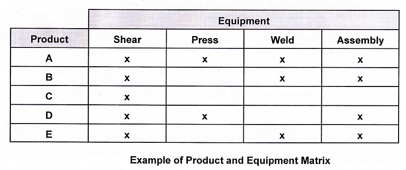


