Some of the Commonly Used Distribution  used in Six Sigma are

1. Normal distribution:

The normal distribution has numerous applications. It is useful when it is equally likely that readings will fall above or below the average. When a sample of several random measurements is averaged, the distribution of such repeated sample averages tends to be normally distributed regardless of the distribution of the measurements being averaged. Mathematically, if

the distribution of (X) bar becomes normal as n increases. If the set of samples being averaged have the same mean and variance, then the mean of the (X) bar is equal to the mean (µ) of the individual measurements, and the variance of the(X) bar is:

Where σ_x², is the variance of the individual variables being averaged. The tendency of sums and averages of independent observations, from populations with finite variances, to become normally distributed as the number of variables being summed or averaged becomes large is known as the central limit theorem. For distributions with little skewness, summing or averaging as few as 3 or 4 variables will result in a normal distribution. For highly skewed distributions, more than 30 variables may have to be summed or averaged to obtain a normal distribution. The normal probability density function is:

The density function shown  is the standard normal probability density  function. The normal probability density function is not skewed The standard normal probability density function has a mean of O and a standard deviation of 1. The normal probability density function cannot be integrated implicitly. Because of this, a transformation to the standard normal distribution is made, and the normal cumulative distribution function or reliability function is read from a table.  If x is a normal random variable, it can be transformed to standard normal using the expression:

Example  A battery is produced with an average voltage of 60 and a standard deviation of 4 volts. If 9 batteries are selected at random, what is the probability that the total voltage of the 9 batteries is greater than 530? What is the probability that 1 the average voltage of the 9 batteries is less than 62?
Solution Part A: The expected total voltage for nine batteries is 540. The expected standard deviation of the voltage of the total of nine batteries is:

S_TOTAL² = 9 x (4)²=144                                                           S_TOTAL=12

Transforming to standard normal: Z = (530-540) /12= -0.833

From the standard normal table, the area to the right of z is 0.7976.

Solution Part B: The expected value is 60. The standard deviation is :

From table P = 0.0668, The area to the left of z is 1 – 0.0668 = 0.9332

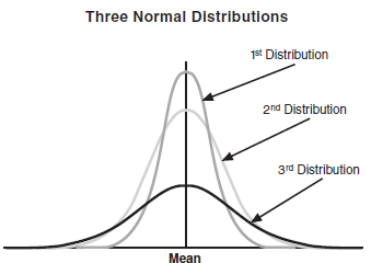
The probability density function of the voltage of the individual batteries and of the average of nine batteries is shown in Figure. The distribution of the averages has less variance because the standard deviation of the averages is equal to the standard deviation of the individuals divided by the square root of the sample size.

When all special causes of variation are eliminated, many variable data processes, when sampled and plotted, produce a bell-shaped distribution. If the base of the histogram is divided into six (6) equal lengths (three on each side of the average), the amount of data in each interval exhibits the following percentages:

The area outside of specification for a normal curve can be determined by a Z value.

The Z transformation formula is:

Where: x = data value (the value of concern)
µ = mean
σ = standard deviation

This transformation will convert the original values to the number of standard deviations away from the mean. The result allows one to use a single standard normal table to describe areas under the curve (probability of occurrence).

There are several ways to display the normal (standardized) distribution:

 1. As a number under the curve up to the Z value:

2. As a number beyond the Z value:

3. As a number under the curve and at a distance from the mean:

2. Binomial Distribution

A binomial distribution is useful when there are only two results in a random experiment (e.g., pass or failure, compliance or noncompliance, yes or no, present or absent). The tool is frequently applicable to attribute data. Altering the first scenario discussed under the normal distribution section to a binomial distribution scenario yields the following:
A dimension on a part is critical . This critical dimension is measured daily on a random sample of parts from a large production process . To expedite the inspection process, a tool is designed to either pass or fail a part that is tested. The output now is no longer continuous. The output is now binary (pass or fail for each part) ; hence, the binomial distribution can be used to develop an attribute sampling plan .
Other application examples are as follows :

• Product either passes or fails test; determine the number of defective units.
• Light bulbs work or do not work; determine the number of defective light bulbs.
• People respond yes or no to a survey question; determine the proportion of people who answer yes to the question.
• Purchase order forms are either filled out incorrectly or correctly; determine the number of transactional errors .
• The appearance of a car door is acceptable or unacceptable ; determine the number of parts of unacceptable appearance .

The following binomial equation could be expressed using either of the following two expressions:

• The probability of exactly x defects in n binomial trials with probability of defect equal to p is [see P(X = x) relationship]
• For a random experiment of sample size n where there are two categories of events, the probability of success of the condition x in one category (where there is n – x in the other category) is

where (q = 1 – p) is the probability that the event will not occur. Also, the binomial coefficient gives the number of possible combinations respect to the number of occurrences, which equates to

From the binomial equation it is noted that the shape of a binomial distribution is dependent on the sample size (n) and the proportion of the population having a characteristic (p) (e.g., proportion of the population that is not in compliance). For an n of 8 and various p values (i.e., 0.1, 0.5, 0.7, and 0.9), the four binomial distributions and corresponding cumulative distributions  (for the probability of an occurrence P), is as:

Example: Consider now that the probability of having the number “2” appear exactly three times in seven rolls of a six-sided die is

we could calculate the probability of “2” occurring for other frequencies besides three out of seven. A summary of these probabilities (e.g., the probability of rolling a “2” one time is 0.390557) is as follows:

P(X =O) = 0.278301
P(X = 1) = 0.390557
P(X = 2) = 0.234897
P(X = 3) = 0.078487
P(X = 4) = 0.015735
P(X = 5) = 0.001893
P(X = 6) = 0.000126
P(X = 7) = 3.62E-06

The probabilities from this table sum to one. From this summary we note that the probability, for example, of rolling a “2” three, four, five, six, or seven times is 0.096245 (i.e., 0.078487 + 0.015735 + 0.001893 + 0.000126 + 3 .62256 x 10-6).

Example:  A part is said to be defective if a hole that is drilled into it is less or greater than specifications . A supplier claims a failure rate of 1 in 100. If this failure rate were true, the probability of observing one defective part in 10 samples is

The probability of the test having a defect is only 0.091 . This exercise has other implications. An organization might choose a sample of 10 to assess a criterion failure rate of 1 in 100. The effectiveness of this test is questionable because the failure rate of the population would need to be a lot larger than 1 / 100 for their to be a good chance of having a defective test sample . That is, the test sample size is not large enough to do an effective job.

 The binomial distribution mean and standard deviation, sigma, can be obtained from the following calculations when the event of interest is the count of defined occurrences in the population, e.g., the number of defectives or effectives.

The binomial mean = µ = np

3. Poisson Distribution

A random experiment of a discrete variable can have several events and the probability of each event is low. This random experiment can follow the Poisson distribution . The following two scenarios exemplify data that can follow a Poisson distribution .
There are a large number of dimensions on a part that are critical. Dimensions are measured on a random sample of parts from a large production process. The number of “out-of-specification conditions” are noted on each sample. This collective “number-of-failures” information from the samples can often be modeled using a Poisson distribution. A repairable system is known to have a constant failure rate as a function of usage (i.e., follows an HPP). In a test a number of systems are exercised and the number of failures are noted for the systems. The Poisson distribution can be used to design /analyze this test. Other application examples are estimating the number of cosmetic nonconformance when painting an automobile, projecting the number of industrial accidents for next year, and estimating the number of unpopped kernels in a batch of popcorn. The Poisson distribution is one of several distributions used to model discrete data and has numerous applications in industry. The Poisson distribution can be an approximation to the binomial when p is equal to or less than 0.1, and the sample size n is fairly larger

where e is a constant of 2.71828, x is the number of occurrences, and λ can equate to a sample size multiplied by the probability of occurrence (i.e., np).nP(X = 0) has application as a Six Sigma metric for yield, which equates to Y = P(X = 0) = e^-λ = e^-D/U = e^-DPU, where D is defects, U is unit, and DPU is defects per unit.

The probability of observing a or fewer events is

The Poisson distribution is dependent only on one parameter, the mean (µ) of the distribution. Figure below shows Poisson distributions (for the probability of an occurrence P) for the mean values of 1, 5, 8, and 10, and corresponding cumulative distributions.

EXAMPLE A company observed that over several years they had a mean manufacturing line shutdown rate of 0.10 per day. Assuming a Poisson distribution, determine the probability of two shutdowns occurring on the same day.
For the Poisson distribution, X. = 0.10 occurrences/day and x = 2 results in the probability P(X = 2) =e^-λλ^x/x!=e^-0.10.1²/2!= 0.004524

The Poisson is used as a distribution for defect counts and can be used as an approximation to the binomial. For np<5, the binomial is better approximated by the Poisson than the normal distribution. When the normalized Poisson is used to model defects, the sample size should be large enough for the Poisson mean to have a value of at least 4 or 5. However, whatever the mean value, the cumulative Poisson distribution provides both the individual and cumulative terms. The Poisson distribution is used to model rates, such as rabbits per acre, defects per unit, or arrivals per hour. The Poisson distribution is closely related to the exponential distribution. If x is a Poisson distributed random variable, then 1/x is an exponential random variable. If x is an exponential random variable, then 1/x is a Poisson random variable. For a random variable to be Poisson distributed, the probability of an occurrence in an interval must be proportional to the length of the interval, and the number of occurrences per interval must be independent.

The Poisson distribution average and standard deviation can be obtained from the following calculations:

4. Chi Square Distribution

The chi-square distribution is an important sampling distribution. One application of this distribution is where the chi-square distribution  is used to determine the confidence interval for the standard deviation of a population. The chi square, t, and F distributions are formed from combinations of random variables. Because of this, they are generally not used to model physical phenomena, like time to fail, but are used to make decisions and construct confidence intervals. These three distributions are considered sampling distributions.
The chi square distribution is formed by summing the squares of standard normal random variables. For example, if z is a standard normal random variable, then:

y=z₁²+z₂²+z₃²+z₄²+….Z_n²

is a chi square random variable (statistic) with n degrees of freedom. A chi square statistic is also created by summing two or more chi square statistics and dividing by the sum of the degrees of freedom. A distribution having this property is regenerative. The chi square distribution is a special case of the gamma distribution with a failure rate of 2, and degrees of freedom equal to 2 divided by the number of degrees of freedom for the corresponding chi square distribution. The chi square probability density function is:

Example: A chi square random variable has 7 degrees of freedom, what is the critical value if 5% of the area under the chi square probability density is desired in the right tail?
Solution : When hypothesis testing, this is commonly referred to as the critical value with 5% significance, or a = 0.05. From the chi square table, this value is 14.067.

5. F Distribution

If X is a chi square random variable with ϒ₁ degrees of freedom, and Y is a chi square random variable with ϒ₂ degrees of freedom, and if X and Y are independent, then:

is an F distribution with ϒ₁ and ϒ₂ degrees of freedom. The F distribution is used extensively to test for equality of variances from two normal populations.

The F probability density function is:

6. Student’s t Distribution

The student’s t distribution is formed by combining a standard normal random variable and a chi square random variable. If z is a standard normal random variable, and X² is a chi square random variable with ϒ degrees of freedom, then a random variable with a t distribution is:

Like the normal distribution, when random variables are averaged, the distribution of the average tends to be normal, regardless of the distribution of the individuals. The t distribution is equivalent to the F distribution with 1 and ϒ degrees of freedom. The t distribution is commonly used for hypothesis testing and constructing  confidence intervals for means. It is used in place of the normal distribution when the standard deviation is unknown. The t distribution compensates for the error in the estimated standard deviation. If the sample size is large, n>100, the error in the estimated standard deviation is small, and the t distribution is approximately normal.
The t probability density function is:

Where ϒ is the degrees of freedom. The t probability density function is as shown

The mean and variance of the t distribution are:

From a random sample of n items, the probability that:

falls between any two specified values is equal to the area under the t probability density function between the corresponding values on the x-axis with n-1 degrees of freedom.

Example: The burst strength of 15 randomly selected seals is given below.
What is the probability that the burst strength of the population is greater than 500?
480    489    491    508    501
500    486    499    479    496
499    504    501    496    498
Solution: The mean of these 15 data points is 495.13. The sample standard deviation of these 15 data points is 8.467. The probability that the population mean is greater than 500 is equal to the area under the t probability density function, with 14 degrees of freedom, to the left of:

From the t table, the area under the t probability density function, with 14 degrees of freedom, to the left of -2.227 is 0.0214. This value must be interpolated (2.227 falls between the 0.025 value of 2.145 and the 0.010 value of 2.624) but can be computed directly using electronic spreadsheets, or calculators. Simply stated, making an inference from the sample of 15 data points, there is a 2.14% possibility that the true population mean is greater than 500.

7. Bivariate Normal Distribution

The joint distribution of two variables is called a bivariate distribution. Bivariate distributions may be discrete or continuous. There may be total independence of the two independent variables, or there may be a covariance between them. The graphical representation of a bivariate distribution is a three dimensional plot, with the x and y-axis representing the independent variables and the z-axis representing the frequency for discrete data or the probability for continuous data. A special case of the bivariate distribution is the bivariate normal distribution, in which there are two random variables. For this case, the bivariate normal density is

Where: µ₁ and µ₂ are the two means
σ₁ and σ₂ are the two variances and are each > 0
ρ is the correlation coefficient of the two random variables
The bivariate normal distribution surface is shown in Figure

Note that the maximum occurs at x1 =µ₁ and x2 =µ₂.

8. Exponential  Distribution

The exponential distribution applies to the useful life cycle of many products. The exponential distribution is used to model items with a constant failure rate. The exponential distribution is closely related to the Poisson distribution. If a random variable, x, is exponentially distributed, then the reciprocal of x, y = 1/x follows a Poisson distribution. Likewise, if x is Poisson distributed, then y = 1/x is exponentially distributed. Because of this behavior, the exponential distribution is usually used to model the mean time between occurrences, such as arrivals or I failures, and the Poisson distribution is used to model occurrences per interval, such as arrivals, failures, or defects.
Where: A is the failure rate and 6 is the mean
From the equation above, it can be seen that A = 1/9.

The following scenario exemplifies a situation that follows an exponential distribution :
A repairable system is known to have a constant failure rate as a function of usage. The time between failures will be distributed exponentially . The failures will have a rate of occurrence that is described by an HPP The Poisson distribution can be used to design a test where sampled systems are tested for the purpose of determining a confidence interval for the failure rate of the system.

The PDF for the exponential distribution is simply f (x) = (1/θ)e^-x/θ
Also f (x) = λe^-λx
From the above equation it can be seen  λ= 1/θ, where λ is the failure rate and θ is the mean

Integration of this equation yields the CDF for the exponential distribution F(x) = 1 – e^-x/θ

The exponential distribution is only dependent on one parameter (θ), which is the mean of the distribution (i.e., mean time between failures). The instantaneous failure rate (i.e., hazard rate) of an exponential distribution is constant and equals 1 /θ. Figure below illustrates the characteristic shape of the PDF, and the corresponding shape for the CDF. The curves were generated for a θ value of 1000.

The variance of the exponential distribution is equal to the mean squared.
σ²= λ²= 1/θ²                               therefore       σ= λ= 1/θ

The exponential distribution is characterized by its hazard function which is constant. Because of this, the exponential distribution exhibits a lack of memory. That is, the probability of survival for a time interval, given survival to the beginning of the interval, is dependent only on the length of the interval.

9. Lognormal Distribution

If a data set is known to follow a lognormal distribution, transforming the data by taking a logarithm yields a data set that is approximately normally distributed.

The most common transformation is made by taking the natural logarithm, but any base logarithm, also yields an approximate normal distribution. When random variables are summed, as the sample size increases, the distribution of the sum becomes a normal distribution, regardless of the distribution of the individuals. Since lognormal random variables are transformed to normal random variables by taking the logarithm, when random variables are multiplied, as the sample size increases, the distribution of the product becomes a lognormal distribution regardless of the distribution of the individuals. This is because the logarithm of the product of several variables is equal to the sum of the logarithms of the individuals. This is shown below:

y = x1  x2  x3 .
ln y=ln x1+ln x2+ln x3

The standard lognormal probability density function is:

Where: µ is the location parameter or mean of the natural logarithms of the individual values
σ is the scale parameter or standard deviation of natural logarithms of the individual values.

The following scenario exemplifies a situation that can follow a lognormal distribution :
A nonrepairable device experiences failures through metal fatigue . Time of failure data from this source often follows the lognormal distribution .

The lognormal distribution exhibits many PDF shapes. This distribution is often useful in the analysis of economic, biological, life data (e.g., metal fatigue and electrical insulation life), and the repair times of equipment. The distribution can often be used to fit data that has a large range of values . The logarithm of data from this distribution is normally distributed; hence, with this transformation, data can be analyzed as if they came from a normal distribution. The lognormal distribution takes on several shapes depending on the value of the shape parameter. The lognormal distribution is skewed right, and the skewness increases as the value of  σ increases.

The mean of the lognormal distribution can be computed from its parameters:

mean = e^{(µ +σ2}/2)

The variance of the lognormal distribution is:

variance = (e^(2µ+σ2))(e^σ2 -1)

Where µ and σ² are the mean and variance of natural log values.

10. Weibull Distribution

The Weibull distribution is one of the most widely used distributions in reliability and  statistical applications. It is commonly used to model time to fail, time to repair, and material strength. There are two common versions of the Weibull distribution, the two parameter Weibull and the three parameter Weibull. The difference is the three parameter Weibull distribution has a location parameter when there is some non- zero time to first failure.
The three parameter Weibull probability density function is:

Where: β is the shape parameter
Θ is the scale parameter
δ is the  location parameter

The three parameter Weibull distribution can also be expressed as:

Where: β is the shape parameter
η is the scale parameter (determines the width of the distribution)
γ is the non-zero location parameter (the point below which there are no failures)

The following scenario exemplifies a situation that can follow a two-parameter Weibull distribution:
A nonrepairable device experiences failures through either early-life, intrinsic, or wear-out phenomena. Failure data of this type often follow the Weibull distribution.

The following scenario exemplifies a situation where a three-parameter Weibull distribution is applicable:

 A dimension on a part is critical . This critical dimension is measured daily on a random sample of parts from a large production process . Information is desired about the “tails” of the distribution . A plot of the measurements indicate that they follow a three-parameter Weibull distribution better than they follow a normal distribution .

The shape parameter is what gives the Weibull distribution its flexibility. By changing the value of the shape parameter, the Weibull distribution can model an, wide variety of data. If β = 1 the Weibull distribution is identical to the exponential distribution, if β = 2, the Weibull distribution is identical to the Rayleigh distribution; if β is between 3 and 4, the Weibull distribution approximates the normal distribution.
The Weibull distribution approximates the lognormal distribution for several values of β. For most populations, more than fifty samples are required to differentiate between the Weibull and lognormal distributions. The effect of the shape parameter on the Weibull distribution is  as shown, the Weibull distribution has shape
flexibility ; hence, this distribution can be used to describe many types of data.

The scale parameter determines the range of the distribution. The scale parameter is also known as the characteristic life if the location parameter is equal to zero. If δ does not equal zero, the characteristic life is equal to Θ+δ; 63.2% of all values fall below the characteristic life regardless of the value of the shape parameter.

The location parameter is used to define a failure-free zone. The probability of failure when x is less than δ is zero. When δ>0, there is a period when no failures can occur. When δ

The mean and variance of the Weibull distribution are computed using the gamma distribution. The mean of the Weibull distribution is equal to the characteristic life if the shape parameter is equal to one.
The mean of the Weibull distribution is:

The variance of the Weibull distribution is:

The variance of the Weibull distribution decreases as the value of the shape parameter increases.

11. Hypergeometric Distribution

The hypergeometric distribution is used to model discrete data. The hypergeometric distribution applies when the population size, N, is small compared to the sample size, or stated another way, when the sample, n, is a relatively large proportion of the population (n >0.1N). Sampling is done without replacement. The hypergeometric distribution is a complex combination calculation and is used when the defined occurrences are known or can be calculated. The number of successes, r, in the sample follows the hypergeometric function:

Where:
N = population size
n = sample size
d = number of occurrences in the population
N – d = number of non occurrences in the population
r = number of occurrences in the sample .
The term x is used instead of r in many texts.

The hypergeometric distribution is similar to the binomial distribution. Both are used to model the number of successes given a fixed number of trials and two possible outcomes on each trial. The difference is that the binomial distribution requires the probability of success to be the same for all trials, while the hypergeometric distribution does not. The hypergeometric distribution using different r values is shown

n = sample size
r = number of occurrences

d = occurrences in population
N = population size

The mean and the variance of the hypergeometric distribution are

Example  From a group of 20 products, 10 are selected at random for testing. What is the probability that the 10 selected contain the 5 best units?
N=20,  n=10, d=5, (N-d)=15 and r=5

Back to Home Page

If you need assistance or have any doubt and need to ask any question  contact at: preteshbiswas@gmail.com. You can also contribute to this discussion and we shall be very happy to publish them in this blog. Your comment and suggestion is also welcome.

Once facts or data have been classified and summarized, they must be interpreted, presented, or communicated in an efficient manner to drive data-based decisions. Statistical problem-solving methods are used to determine if processes are on target if the total variability is small compared to specifications and if the process is stable over time. Businesses can no longer afford to make decisions based on averages alone; process variations and their sources must be identified and eliminated.

Descriptive statistics are used to describe or summarize a specific collection of data (typical samples of data). Descriptive statistics encompass both numerical and graphical techniques, and are used to determine the:

• The central tendency of the data.
• Spread or dispersion of the data.
• Symmetry and skewness of the data.

Inferential statistics is the method of collecting samples of data and making inferences about population parameters from the sample data. Before reviewing basic statistics, the different types of data must be identified. The type of data that has been collected as process inputs (x’s) and/or outputs (y’s) will determine the type of statistics or analysis that can be performed.

Types of Data

Data is objective information that everyone can agree on. Measurability is important in collecting data. The three types of data are attribute data, variables data, and locational data. Of these three, attribute and variables data are more widely used.
Attribute data is discrete. This means that the data values can only be integers, for example, 3, 48, 1029. Counted data or attribute data are answers to questions like “how many”, “how often”, or “what kind.” Examples include:

• How many of the final products are defective?
• How many people are absent each day?
• How many days did it rain last month?
• What kind of performance was achieved?

Variables data is continuous. This means that the data values can be any real number, for example, 1.037, -4.69, 84.35. Measured data (variables data) are answers to questions like “how long,” “what volume,” “how much time” and “how far.” This data is generally measured with some instrument or device. Examples include:

• How long is each item?
• How long did it take to complete the task?
• What is the weight of the product?

Measured data is regarded as being better than counted data. It is more precise and contains more information. For example, one would certainly know much more about the climate of an area if they knew how much it rained each day rather than how many days trained. Collecting measured data is often difficult or expensive, so counted data must be used. In some situations, data will only occur as counted data. For example, a food producer may measure the performance of microwave popcorn by counting the number of unpropped kernels of corn in each bag tested. For information that can be obtained as either attribute or variables data, it is generally preferable to collect variables data.

The third type of data which does not fit into attribute data and variable  data is known as locational data which simply answers the question “where.” Charts that utilize locational data are often called “measles charts” or concentration charts. Examples are a drawing showing locations of paint blemishes on an automobile or a map of Pune with sales and distribution offices indicated.

Another way to classify data is as discrete or continuous.

Continuous data:

• Has no boundaries between adjoining values.
• Includes most non-counting intervals and ratios(e.g., time).

Discrete data:

• Has clear boundaries.
• Includes nominals, counts, and rank-orders, (e.g., Monday vs. Friday, an electrical circuit with or without a short).

Conversion of Attributes Data to Variables Measures

Some data may only have discrete values, such as this part is good or bad, or I like or dislike the quality of this product. Since variables data provides more information than does attribute data, for a given sample size, it is desirable to use variables data whenever possible. When collecting data, there are opportunities for some types of data to be either attributes or variables. Instead of a good or bad part, the data can be stated as to how far out of tolerance or within tolerance it is. The like or dislike of product quality can be converted to a scale of how much do I like or dislike it.

Referring back to the Table above, two of the data examples could easily be presented as variables data: 10 scratches could be reported as the total scratch length of 8.37 inches, and 25 paint runs as 3.2 sq. in. surface area of paint runs. Consideration of the cost of collecting variables versus attributes data should also be given when choosing the method. Typically, the measuring instruments are more costly for performing variables measurements, and the cost to organize, analyze and store variables data is higher as well. A go/no-go ring gage can be used to quickly check outside diameter threads. To determine the actual pitch diameter is a slower and more costly process. Variables data requires storing of individual values and computations for the mean, standard deviation, and other estimates of the population. Attributes data requires minimal counts of each category and hence requires very little data storage space. For manual data collection, the required skill level of the technician is higher for variables data than for attribute data. Likewise, the cost of automated equipment for variables data is higher than for attributes data. The ultimate purpose for the data collection and the type of data are the most significant factors in the decision to collect attribute or variables data.

The table details the four Measurement scales in increasing order of statistical desirability.

 Many of the interval measures may be useful for ratio data as well.

Examples of continuous data, discrete data, and measurement scales:

1.  Continuous data:  A Wagon weighs 478.61 Kg
2. Discrete data: Of a lot, 400 pieces failed
3. Ordinal scale: Defects are categorized as critical, major A, major B, and minor
4. Nominal scale: A print-out of all shipping codes for last week’s orders
5. Ratio scale: The individual weights of a sample of widgets
6. Interval scale: The temperatures of steel rods (°F) after one hour of cooling

Ensuring Data Accuracy and Integrity.

Bad data is not only costly to capture but corrupts the decision-making process.  Some considerations include:

• Avoid emotional bias relative to targets or tolerances when counting, measuring, or recording digital or analogue displays.
• Avoid unnecessary rounding. Rounding often reduces measurement
  sensitivity. Averages should be calculated to at least one more decimal position than individual readings.
• If data occurs in time sequence, record the order of its capture.
• If an item characteristic changes over time, record the measurement or classification as soon as possible after its manufacture, as well as after a stabilization period.
• To apply statistics which assume a normal population, determine whether the expected dispersion of data can be represented by at least 8 to 10 resolution increments. If not, the default statistic may be the count of observations which do or do not meet specification criteria.
• Screen or filter data to detect and remove data entry errors such as digital transposition and magnitude shifts due to a misplaced decimal point.
• Avoid removal by hunch. Use objective statistical tests to identify outliers.
• Each important classification identification should be recorded along with the data. This information can include time, machine, auditor, operator, gage, lab, material, target, process change and conditions, etc.

It is important to select a sampling plan appropriate for the purpose of the use of the data. There are no standards as to which plan is to be used for data collection and analysis, therefore the analyst makes a decision based upon experience and the specific needs. There are many other sampling techniques that have been developed for specific needs.

Population vs. Sample

A population is every possible observation or census, but it is very rare to capture the entire population in data collection. Instead, samples, or subsets of populations as illustrated in the following figure, are captured. A statistic, by definition, is a number that describes a sample characteristic. Information from samples can be used to “infer” or approximate a population characteristic called a parameter.

1. Random Sampling

   Sampling is often undertaken because of time and economic advantages. The use of a sampling plan requires randomness in sample selection. Obviously, true random sampling requires giving every part an equal chance of being selected for the sample. The sample must be representative of the lot and not just the product that is easy to obtain. Thus, the selection of samples requires some upfront thought and planning. Often, the emphasis is placed on the mechanics of sampling plan usage and not on sample identification and selection. Sampling without randomness ruins the effectiveness of any plan. The product to be sampled may take many forms: in a layer, on a conveyor, in sequential order, etc. The sampling sequence must be based on an independent random plan. The sample is determined by selecting an appropriate number from a hat or random number table.

2. Sequential Sampling

   Sequential sampling plans are similar to multiple sampling plans except that sequential sampling can theoretically continue indefinitely. Usually, these plans are ended after the number inspected has exceeded three times the sample size of a corresponding single sampling plan. Sequential testing is used for costly or destructive testing with sample sizes of one and is based on a probability ratio test developed by Wald .

3. Stratified Sampling

   One of the basic assumptions made in sampling is that the sample is randomly selected from a homogeneous lot. When sampling, the “lot” may not be homogeneous. For example, parts may have been produced on different lines, by different machines, or under different conditions. One product line may have well-maintained equipment, while another product line may be older or have poorly %  maintained equipment. The concept behind stratified sampling is to attempt to select random samples from each group or process that is different from other similar groups or processes. The resulting mix of samples thus drawn can be biased if the proportion of the samples does not reflect the relative frequency of the groups. To the person using the sample data, the implication is that they must first be aware of the possibility of stratified groups and second, phrase the data report such that the observations are relevant only to the sample drawn and may not necessarily reflect the overall system.

Data Collection Methods

Collecting information is expensive. To ensure that the collected data is relevant to the problem, some prior thought must be given to what is expected. Manual data collection requires a data form. Check sheets, tally sheets, and checklists are data collection methods that are widely used. Other data collection methods include automatic measurement and data coding.
Some data collection guidelines are:

• Formulate a clear statement of the problem
• Define precisely what is to be measured
• List all the important characteristics to be measured
• Carefully select the right measurement technique
• Construct an uncomplicated data form
• Decide who will collect the data
• Arrange for an appropriate sampling method
• Decide who will analyze and interpret the results
• Decide who will report the results

Without an operational definition, most data is meaningless. Both attribute and variable specifications must be defined. Data collection includes both manual and automatic methods. Data collected manually may be done using printed forms or by data entry, at the time the measurements are taken. Manual systems are labor-intensive and subject to human errors in measuring and recording the correct values. Automatic data collection includes electronic chart recorders and digital storage. The data collection frequency may be synchronous, based on a set time interval, or asynchronous, based on events. Automatic systems have higher initial costs than manual systems and have the disadvantage of collecting both “good” and “erroneous” data. Advantages to using automatic data collection systems include high accuracy rates and the ability to operate unattended.

Automatic Measurement

Automatic sorting gages are widely used to sort parts by dimension. They are normally accurate within 0.0001″. When computers are used as part of an automated measurement process, there are several important issues. Most of these stem from the requirements of software quality engineering but have important consequences in terms of ensuring that automated procedures get answers at least as “correct” as those that arise from manual measurements. Computer-controlled measurement systems may offer distinct advantages over their human counterparts. (Examples include improved test quality, shorter inspection times, lower operating costs, automatic report generation, improved accuracy, and automatic calibration.) Automated measurement systems have the capacity and speed to be used in high-volume operations. Automated systems have the disadvantages of higher initial costs, and a lack of mobility and flexibility compared to humans. Automated systems may require technical malfunction diagnostics. When used properly, they can be a powerful tool to aid in the improvement of product quality. Applications for automatic measurement and digital vision systems are quite extensive. The following incomplete list is intended to show examples:

• Error proofing a process
• Avoiding human boredom and errors
• Sorting acceptable from defective parts
• Detecting flaws, surface defects, or foreign material
• Creating CAD drawings from an object
• Building prototypes by duplicating a model
• Making dimensional measurements
• Performing high-speed inspection of critical parameters
•  Machining, using either laser or mechanical methods
• Marking and identifying parts
• Inspecting solder joints on circuit boards
• Verifying and inspecting the packaging
• Providing optical character and bar code recognition
• Identifying missing components
• Controlling motion
• Assembling components
• Verifying colour

Data Coding

The efficiency of data entry and analysis is frequently improved by data coding. Problems due to not coding include:

• Inspectors trying to squeeze too many digits into small blocks on a form
• Reduced throughput and increased errors by clerks at keyboards reading and entering large sequences of digits for a single observation
• insensitivity of analytic results due to rounding large sequences of digits

Coding by adding or subtracting a constant or by multiplying or dividing by a factor:

Let the subscript, lowercase c, represent a coded statistic; the absence of a subscript represents raw data; uppercase C indicates a constant, and lowercase f represents a factor. Then:

Coding by substitution:

Consider a dimensional inspection procedure in which the specification is nominal plus and minus 1.25″. The measurement resolution is 1/8 of an inch and inspectors, using a ruler, record plus and minus deviations from nominal. A typically recorded observation might be 32-3/8″ crammed in a space that was designed to accommodate three characters. The data can be coded as integers expressing the number of 1/8 inch increments deviating from nominal. The suggestion that check sheet blocks could be made larger could be countered by the objection that there would be fewer data points per page.

Coding by truncation of repetitive place values:

Measurements such as 0.55303, 0.55310, 0.55308, in which the digits 0.553 repeats in all observations, can be recorded as the last two digits expressed as integers. Depending on the objectives of the analysis, it may or may not be necessary to decode the measurements.

Probability

Most quality theories use statistics to make inferences about a population based on information contained in samples. The mechanism one uses to make these inferences is probability.

Conditions for Probability

The probability of any event, E, lies between 0 and 1. The sum of the probabilities of all possible events in a sample space, S, = 1.

Simple Events

An event that cannot be decomposed is simple, E. The set of all sample points for an experiment is called the sample space, S.
If an experiment is repeated a large number of times, N, and the event, E, is observed n_E times, the probability of E is approximate:

For eg the probability of observing 3 on the toss of a single die is:

 What is the probability of getting 1, 2, 3, 4, 5, or 6 by throwing a die?

Use of Venn (Circle) Diagrams

A Venn diagram or set diagram is a diagram that shows all possible logical relations between a finite collection of different sets. Venn diagrams were conceived around 1880 by John Venn. They are used to teach elementary set theory, as well as illustrate simple set relationships in probability, logic, statistics, linguistics, and computer science. On occasion, a circle diagram can help conceptualize the relationship between work elements in order to optimize work activities. Shown below is a hypothetical analysis of the workload for a shipping employee using a Venn (or circle) diagram.

 A Venn (circle) diagram illustrates relationships between events. In this case, there is an overlap between packing and data entry, as well as packing and pulling stock. Making CDs is exclusive of other activities. If the sample space equals 1.0 or 100%, then one can determine both the busy time and idle time in an 8-hour shift.
Busy time = Packing + Data entry + Pulling stock + Making CDs – Overlap
= 0.30 + 0.20 + 0.25 + 0.10 – 0.06 – 0.04
= 0.85 – 0.10
= 0.75

In an 8-hour shift, there are 6.0 hours of activity. By the same logic, there are 2.0 idle hours. After deducting customary lunch and break times, one can consider whether additional duties can be assumed by this individual.  Venn diagrams are normally used to explain probability theory. In the above diagram, making CDs and packing are mutually exclusive, but packing and pulling stock are not. The final calculation is reflected in ‘the additive law of probability

Compound Events

Compound events are formed by a composition of two or more events. They consist of more than one point in the sample space. For example, if two dice are tossed, what is the probability of getting an 8? A die and a coin are tossed. What is the probability of getting a 4 and tail? The two most important probability theorems are additive and multiplicative. For the following discussion, E_A = A and E_B = B.

l. Composition.

Consists of two possibilities -a union or intersection.

A. Union of A and B

If A and B are two events in a sample space, S, the union of A and B (A U B) contains all sample points in events A, B, or both.

Example:  In the die toss E₁,E₂,E₃,E₄,E₅ and E₆ is probability of getting 1, 2, 3, 4, 5, or 6, consider the following:
If A = E₁, E₂ and E₃ (numbers less than 4)
and B = E₁, E₃ and E₅ (odd numbers),
then A U B = E₁, E₂, E₃ and E₅.

B. Intersection of A and B

If A and B are two events in a sample space, S, the intersection of A and B (A ∩ B) is composed of all sample points that are in both A and B.
From the above example, A ∩ B = E₁  and  E₃

ll. Event Relationships.

There are three relationships involved in finding the probability of an event: complementary, conditional, and mutually exclusive.

A. Complement of an Event

The complement of event A is all sample points in the sample space, S, but not in A. The complement of A is 1-P_A.
For Example, If P_A (cloudy days) is 0.3, the complement of A would be 1 – P_A = 0.7 (clear).

B. Conditional Probabilities

The conditional probability of event A occurring, given that event B, has occurred is:

For example, If event A (rain) = 0.2 and event B (cloudiness) = 0.3, what is the probability of rain on a cloudy day? (Note, it will not rain without clouds.)

Two events A and B are said to be independent if either:
P(A|B) = P(A) or P(B|A) = P(B)
However, P(A|B) = 0.67 and P(A) = 0.2= no equality, and
P(B|A) = 1.00 and P(B) = 0.3 = no equality.
Therefore, the events are said to be dependent.

C. Mutually Exclusive Events

If event A contains no sample points in common with event B, then they are said to be mutually exclusive.
For Example, Obtaining a 3 and a 2 on the toss of a single die is a mutually exclusive event. The probability of observing both events simultaneously is zero.
The probability of obtaining either a 3 or a 2 is:
PE₂+PE₃=1/6 + 1/6= 1/3

1. The Additive Law

   1. If the two events are not mutually exclusive:
      P(A U B)=P(A)+P(B)-P(A|B)
      Note that P (A U B) is shown in many texts as P (A + B) and is read as the probability of A or B.

      For Example, If one owns two cars and the probability of each car starting on a cold morning is 0.7, what is the probability of getting to work on his car?

      

P (A U B) = 0.7 + 0.7 – (0.7×0.7)
=1.4 – 0.49 =0.91 or 91%

1. If the two events are mutually exclusive, the law reduces to:
   P (A U B) = P(A) + P(B) also P (A + B) = P(A) + P(B)

   For Example, If the probability of finding a black sock in a dark room is 0.4 and the probability of finding a blue sock is 0.3, what is the chance of finding a blue or black sock?

    

P (A U B) = 0.4 + 0.3 = 0.7 or  70%

Note: The problem statements centre around the word “or”
Will car A or B start?
Will one get a black or blue sock?

For any two events, A and B, such that P(B) ≠ 0:
P(A|B) = P(A ∩ B)/ P(B) and P(A ∩ B) = P(A|B)P(B)

Note: The problem statements center around the word “and”

Descriptive Statistics

Descriptive statistics include measures of central tendency, measures of dispersion, probability density function, frequency distributions, and cumulative distribution functions.

Measures of Central Tendency

Measures of central tendency represent different ways of characterizing the central value of a collection of data. Three of these measures will be addressed here: mean, mode, and median.

The Mean X̅̅ (X -bar)

The mean is the total of all data values divided by the number of data points.

For Example The    for the following 9 numbers, 5 3 7 9 8 5 4 5 8 is 6

The arithmetic mean is the most widely used measure of central tendency.

Advantages of using the mean:

• It is the centre of gravity of the data
• It uses all data
• No sorting is needed

Disadvantages of using the mean:

• Extreme data values may distort the picture
• It can be time-consuming
• The mean may not be the actual value of any data points,

The Mode

The mode is the most frequently occurring number in a data set.
For Eg . the mode of the following data set: 5 3 7 9 8 5 4 5 8  is: 5
Note: It is possible for groups of data to have more than one mode.

Advantages of using the mode:

• No calculations or sorting are necessary
• It is not influenced by extreme values A
• It is an actual value
• it can be detected visually in distribution plots

The disadvantage of using the mode:

• The data may not have a mode or may have more than one mode

The Median (Midpoint)

The median is the middle value when the data is arranged in ascending or descending order. For an even set of data, the median is the average of the middle two values.
Examples: Find the median of the following data set:
(10 Numbers) 2 2 2 3 4 6 7 7 8 9
(9 Numbers) 2 2 3 4 5 7 8 8 9
Answer: 5 for both examples

Advantages of using the median:

• Provides an idea of where most data is located
• Little calculation required
• insensitivity to extreme values

Disadvantages of using the median:

• The data must be sorted and arranged
• Extreme values may be important.
• Two medians cannot be averaged to obtain a combined distribution median
• The median will have more variation (between samples) than the average

 Measures of Dispersion

Other than the central tendency, the other important parameter to describe a set of data is spread or dispersion. Three main measures of dispersion will be reviewed: range, variance, and standard deviation.

 Range (R)

The range of a set of data is the difference between the largest and smallest values.
Example  Find the range of the following data set: 5 3 7 9 3 5 4 5 3
Answer: 9 – 3 = 6

 Variance ( σ²,s²)

The variance, σ² or s², is equal to the sum of the squared deviations from the mean, divided by the sample size. The formula for variance is:

The variance is equal to the standard deviation squared.

 Standard Deviation (σ, s)

The standard deviation is the square root of the variance.

Alternatively

N is used for a population and n -1 for a sample to remove potential bias in relatively small samples (less than 30).

Example: Calculate the Standard Deviation of the following Data set using the formula

Coefficient of Variation (COV)

The coefficient of variation equals the standard deviation divided by the mean and is expressed as a percentage. 

Probability Density Function

In probability theory, a probability density function (PDF), or density of a continuous random variable, is a function that describes the relative likelihood for this random variable to take on a given value. The probability of the random variable falling within a particular range of values is given by the integral of this variable’s density over that range—that is, it is given by the area under the density function but above the horizontal axis and between the lowest and greatest values of the range. The probability density function is nonnegative everywhere, and its integral over the entire space is equal to one.

Suppose a species of bacteria typically lives 4 to 6 hours. What is the probability that a bacterium lives exactly 5 hours? The answer is actually 0%. Lots of bacteria live for approximately 5 hours, but there is a negligible chance that any given bacterium dies at exactly 5.0000000000.. hours. Instead, we might ask: What is the probability that the bacterium dies between 5 hours and 5.01 hours? Let’s say the answer is 0.02 (i.e., 2%). Next: What is the probability that the bacterium dies between 5 hours and 5.001 hours? The answer is probably around 0.002 since this is 1/10th of the previous interval. The probability that the bacterium dies between 5 hours and 5.0001 hours is probably about 0.0002, and so on. The ratio (probability of dying during an interval) / (duration of the interval) is approximately constant and equal to 2 per hour (or 2 /hour). For example, there is 0.02 probability of dying in the 0.01-hour interval between 5 and 5.01 hours, and (0.02 probability / 0.01 hours) = 2 /hour. This quantity 2/ hour is called the probability density for dying at around 5 hours.

Therefore, in response to the question “What is the probability that the bacterium dies at 5 hours?”, a literally correct but unhelpful answer is “0”, but a better answer can be written as (2/ hour) dt. This is the probability that the bacterium dies within a small (infinitesimal) window of time around 5 hours, where it is the duration of this window. For example, the probability that it lives longer than 5 hours but shorter than (5 hours + 1 nanosecond), is (2/hour)×(1 nanosecond) ≃ 6×10−13 (using the unit conversion 3.6×1012 nanoseconds = 1 hour). There is a probability density function f with f(5 hours) = 2/ hour. The integral of f over any window of time (not only infinitesimal windows but also large windows) is the probability that the bacterium dies in that window.

The probability density function, f(x), describes the behaviour of a random variable. Typically, the probability density function is viewed as the “shape” of the distribution. It is normally a grouped frequency distribution. Consider the histogram for the length of a product shown in Figure below.

A histogram is an approximation of the distribution’s shape. The histogram shown appears symmetrical. It shows this histogram with a smooth curve overlaying the data. The smooth curve is the statistical model that describes the population; in this case, the normal distribution.
When using statistics, the smooth curve represents the population. The differences between the sample data represented by the histogram and the population data represented by the smooth curve are assumed to be due to sampling error. In reality, the difference could also be caused by a lack of randomness in the sample or an incorrect model. The probability density function is similar to the overlaid model. The area below the probability density function to the left of a given value, x, is equal to the probability of the random variable represented on the x-axis is less than the given value x. Since the probability density function represents the entire sample space, the area under the probability density function must equal one. Since negative probabilities are impossible, the probability density function, f(x), must be positive for all values of x.
Stating these two requirements mathematically for continuous distributions with f(x)≥ 0;

The figure below demonstrates how the probability density function is used to compute probabilities. The area of the shaded region represents the probability of a single product drawn randomly from the population having a length less than 185. This probability is 15.9% and can be determined by using the standard normal table.

Cumulative Distribution Function

The cumulative distribution function, F(x), denotes the area beneath the probability density function to the left of x.

The area of the shaded region of the probability density function is 0.2525 which corresponds to the cumulative distribution function at x = 190. Mathematically, the cumulative distribution function is equal to the integral of the probability density function to the left of x.

For Example, A random variable has the probability density function f(x) = 0.125x, where x is valid from 0 to 4. The probability of x being less than or equal to 2 is:

Properties of a Normal Distribution

A normal distribution can be described by its mean and standard deviation. The standard normal distribution is a special case of the normal distribution and has a mean of zero and a standard deviation of one. The tails of the distribution extend to ± infinity. The area under the curve represents 100% of the possible observations. The curve is symmetrical such that each side of the mean has the same shape and contains 50% of the total area. Theoretically, about 95% of the population is contained within ± 2 standard deviations.

If a data set is normally distributed, then the standard deviation and mean can be used to determine the percentage (or probability) of observations within a selected range. Any normally distributed scale can be transformed to its equivalent Z scale or score using the formula:   Z= (x-μ)/σ
x will often represent a lower specification limit (LSL) or upper specification limit (USL). Z, the “sigma value,” is a measure of standard deviations from the mean. Any normal data distribution can be transformed to a standard normal curve using the Z transformation. The area under the curve is used to predict the probability of an event occurring.

Example: If the mean is 85 days and the standard deviation is five days, what would be the yield if the USL is 90 days?

A standard Z table is used to determine the area under the curve. The area under the curve represents probability.

Because the curve is symmetric, the area shown as yield would be 1-P(z>1) = 0.841 or 84.1%.
In accordance with the equation, Z can be calculated for any “point of interest,” x.

Variation

The following figure shows three normal distributions with the same mean. What differs between the distributions is the variation.

The first distribution displays less variation or dispersion about the mean. The second distribution displays more variation and would have a greater standard deviation. The third distribution displays even more variation.

Short-term vs. Long-term Variation

The duration over which data is collected will determine whether short-term or long-term variation has been captured within the subgroup.
There are two types of variation in every process:
common cause variation and special cause variation. Common cause variation is completely random (i.e., the next data point’s specific value cannot be predicted). It is the natural variation of the process. Special cause variation is the nonrandom variation in the process. It is the result of an event, an action, or a series of events or actions. The nature and causes of special cause variation are different for every process. Short-term data is data that is collected from the process in subgroups. Each subgroup is collected over a short length of time to capture common cause variation only (i.e., data is not collected across different shifts because variation can exist from operator to operator).
Thus, the subgroup consists of “like” things collected over a narrow time frame and is considered a “snapshot in time” of the process. For example, a process may use several raw materials lots per shift. A representative short-term sample may consist of CTQ measurements within one lot. Long-term data is considered to contain both special and common causes of variation that are typically observed when all of the input variables have varied over their full range. To continue with the same example, long-term data would consist of several raw material lots measured across several short-term samples.

Processes tend to exhibit more variation in the long term than in the short term. Long-term variability is made up of short-term variability and process drift. The shift from short term to long term can be quantified by taking both short-term and long-term samples.

On average, short-term process means tend to shift and drift by 1.5 sigmas.
Z_lt = Z_st – 1.5
(The short-term Z (Z_st) is also known as the benchmark sigma value. A Six Sigma process would have six standard deviations between the mean and the closest specification limit for a short-term capability study. The following figure illustrates the Z-score relationship to the Six Sigma philosophy:

In a Six Sigma process, customer satisfaction and business objectives are robust to shifts caused by process or product variation.

Drawing Valid Statistical Conclusions

The objective of statistical inference is to draw conclusions about population characteristics based on the information contained in a sample. Statistical inference in a practical situation contains two elements: (1) the inference and (2) a measure of its validity. The steps involved in statistical inference are:

• Define the problem objective precisely
• Decide if the problem will be evaluated by a one-tail or two-tail test
•  Formulate a null hypothesis and an alternate hypothesis
• Select a test distribution and a critical value of the test statistic reflecting the degree of uncertainty that can be tolerated (the alpha, α, risk)
• Calculate a test statistic value from the sample information
•  Make an inference about the population by comparing the calculated value to the critical value. This step determines if the null hypothesis is to be rejected. If the null is rejected, the alternate must be accepted.
•  Communicate the findings to interested parties

Every day, in our personal and professional lives, individuals are faced with decisions between choice A or choice B. In most situations, the relevant information is available, but it may be presented in a form that is difficult to digest. Quite often, the data seems inconsistent or contradictory. In these situations, an intuitive decision may be little more than an outright guess. While most people feel their intuitive powers are quite good, the fact is that decisions made on gut-feeling are often wrong.

Null Hypothesis and Alternative Hypothesis

The null hypothesis is the hypothesis to be tested. The null hypothesis directly stems from the problem statement and is denoted as H_o;
The alternate hypothesis must include all possibilities which are not included in the null hypothesis and is designated H₁.
Examples of null and alternate hypothesis: :
Null hypothesis            : H_o: Y_a = Y_b                            H_o: A ≤ B
Alternate hypothesis: H_o: Y_a ≠ Y_b                            H_o: A > B

A null hypothesis can only be rejected, or fail to be rejected, it cannot be accepted because of a lack of evidence to reject it.

Add Test Statistic

In order to test a null hypothesis, a test calculation must be made from sample information. This calculated value is called a test statistic and is compared to an appropriate critical value. A decision can then be made to reject or not reject the null hypothesis.

Types of Errors

When formulating a conclusion regarding a population-based on observations from a small sample, two types of errors are possible:

• Type I error: This error results when the null hypothesis is rejected when it is, in fact, true.
• Type II error: This error results when the null hypothesis is not rejected when it should be rejected.

The degree of risk (α) is normally chosen by the concerned parties (α is normally taken as 5%) in arriving at the critical value of the test statistic.

Enumerative (Descriptive) Studies

Enumerative data is data that can be counted. For example the classification of things, the classification of people into intervals of income, age, health. A census is an enumerative collection and study. Useful tools for tests of hypothesis conducted on enumerative data are the chi-square, binomial, and Poisson distributions. Deming, in 1975, defined contrast between enumeration and analysis:

• Enumerative study: A study in which action will be taken on the universe.
• An analytical study: A study in which action will be taken on a process to improve performance in the future.

Numerical descriptive measures create a mental picture of a set of data. The measures calculated from a sample are called statistics. When these measures describe a population, they are called parameters.

The table shows examples of statistics and parameters for the mean and standard deviation. These two important measures are called central tendency and dispersion.

Summary of Analytical and Enumerative Studies

Analytical studies start with the hypothesis statement made about population parameters. A sample statistic is then used to test the hypothesis and either reject or fail to reject the null hypothesis. At a stated level of confidence, one is then able to make inferences about the population.

Back to Home Page

If you need assistance or have any doubt and need to ask any question contact me at preteshbiswas@gmail.com. You can also contribute to this discussion and I shall be happy to publish them. Your comment and suggestion are also welcome.

What is Six Sigma?

• As per Jack welch “Six Sigma is a quality program that, when all is said and done, improves your customer’s experience, lowers your costs, and builds better leaders.”
• Six Sigma is simply a method of efficiently solving a problem. Using Six Sigma reduces the amount of defective products manufactured or services provided, resulting in increased revenue and greater customer satisfaction.
• Six Sigma is a method that provides organizations tools to improve the capability of their business processes. This increase in performance and decrease in process variation lead to defect reduction and improvement in profits, employee morale, and quality of products or services. Six Sigma quality is a term generally used to indicate a process is well controlled (within process limits ±3s from the center line in a control chart, and requirements/tolerance limits ±6s from the center line).  Different definitions have been proposed for Six Sigma, but they all share some common threads:
  • Use of teams that are assigned well-defined projects that have direct impact on the organization’s bottom line.
  • Training in “statistical thinking” at all levels and providing key people with extensive training in advanced statistics and project management. These key people are designated “Black Belts.” Review the different Six Sigma belts, levels and roles.
  • Emphasis on the DMAIC approach to problem solving: define, measure, analyze, improve, and control.
  • A management environment that supports these initiatives as a business strategy.

Six Sigma offers six major benefits that attract companies:

• Generates sustained success
• Sets a performance goal for everyone
• Enhances value to customers
• Accelerates the rate of improvement
• Promotes learning and cross-pollination
• Executes strategic change

What exactly does “Six Sigma” mean?

Six Sigma is named after a statistical concept where a process only produces 3.4 defects per million opportunities (DPMO). Six Sigma can therefore be also thought of as a goal, where processes not only encounter less defects, but do so consistently (low variability). Basically, Six Sigma reduces variation, so products or services can be delivered as expected reliably.

Six sigma: Statistically visualized

Differing opinions on the definition of Six Sigma:

• Philosophy — The philosophical perspective views all work as processes that can be defined, measured, analyzed, improved and controlled. Processes require inputs (x) and produce outputs (y). If you control the inputs, you will control the outputs. This is generally expressed as y = f(x).
• Set of tools — The Six Sigma expert uses qualitative and quantitative techniques to drive process improvement. A few such tools include statistical process control (SPC), control charts, failure mode and effects analysis, and process mapping. Six Sigma professionals do not totally agree as to exactly which tools constitute the set.
• Methodology — This view of Six Sigma recognizes the underlying and rigorous approach known as DMAIC (define, measure, analyze, improve and control). DMAIC defines the steps a Six Sigma practitioner is expected to follow, starting with identifying the problem and ending with the implementation of long-lasting solutions. While DMAIC is not the only Six Sigma methodology in use, it is certainly the most widely adopted and recognized.
• Metrics – In simple terms, Six Sigma quality performance means 3.4 defects per million opportunities (accounting for a 1.5-sigma shift in the mean).

Features of Six Sigma

Six Sigma’s aim is to eliminate waste and inefficiency, thereby increasing customer satisfaction by delivering what the customer is expecting. Six Sigma follows a structured methodology and has defined roles for the participants. Six Sigma is a data driven methodology and requires accurate data collection for the processes being analyzed. Six Sigma is about putting results on Financial Statements. Six Sigma is a business-driven, multi-dimensional structured approach for:

• Improving Processes
• Lowering Defects
• Reducing process variability
• Reducing costs
• Increasing customer satisfaction
• Increased profits

The word Sigma is a statistical term that measures how far a given process deviates from perfection. The central idea behind Six Sigma: If you can measure how many “defects” you have in a process, you can systematically figure out how to eliminate them and get as close to “zero defects” as possible and specifically it means a failure rate of 3.4 parts per million or 99.9997% perfect.

The statistical representation of Six Sigma describes quantitatively how a process is performing. To achieve Six Sigma, a process must not produce more than 3.4 defects per million opportunities. A Six Sigma defect is defined as anything outside of customer specifications. A Six Sigma opportunity is then the total quantity of chances for a defect. Process sigma can easily be calculated using a Six Sigma calculator. The fundamental objective of the Six Sigma methodology is the implementation of a measurement-based strategy that focuses on process improvement and variation reduction through the application of Six Sigma improvement projects. This is accomplished through the use of two Six Sigma sub-methodologies: DMAIC and DMADV. The Six Sigma DMAIC process (define, measure, analyze, improve, control) is an improvement system for existing processes falling below specification and looking for incremental improvement. The Six Sigma DMADV process (define, measure, analyze, design, verify) is an improvement system used to develop new processes or products at Six Sigma quality levels. It can also be employed if a current process requires more than just incremental improvement. Both Six Sigma processes are executed by Six Sigma Green Belts and Six Sigma Black Belts and are overseen by Six Sigma Master Black Belts. According to the Six Sigma Academy, Black Belts save companies approximately $230,000 per project and can complete four to six projects per year. (Given that the average Black Belt salary is $80,000 in the United States, that is a fantastic return on investment.) General Electric, one of the most successful companies implementing Six Sigma, has estimated benefits on the order of $10 billion during the first five years of implementation. GE first began Six Sigma in 1995 after Motorola and Allied Signal blazed the Six Sigma trail. Since then, thousands of companies around the world have discovered the far-reaching benefits of Six Sigma. Many frameworks exist for implementing the Six Sigma methodology. Six Sigma Consultants all over the world have developed proprietary methodologies for implementing Six Sigma quality, based on the similar change management philosophies and applications of tools.

Key Concepts of Six Sigma

At its core, Six Sigma revolves around a few key concepts.

• Critical to Quality: Attributes most important to the customer.
• Defect: Failing to deliver what the customer wants.
• Process Capability: What your process can deliver.
• Variation: What the customer sees and feels.
• Stable Operations: Ensuring consistent, predictable processes to improve what the customer sees and feels.
• Design for Six Sigma: Designing to meet customer needs and process capability.
  Our Customers Feel the Variance, Not the Mean. So Six Sigma focuses first on reducing process variation and then on improving the process capability.

Myths about Six Sigma

There are several myths and misunderstandings surrounding Six Sigma. Some of them are given below:

• Six Sigma is only concerned with reducing defects.
• Six Sigma is a process for production or engineering.
• Six Sigma cannot be applied to engineering activities.
• Six Sigma uses difficult-to-understand statistics.
• Six Sigma is just training.

Origin of Six Sigma

• Six Sigma originated at Motorola in the early 1980s, in response to achieving 10X reduction in product-failure levels in 5 years.
• Engineer Bill Smith invented Six Sigma, but died of a heart attack in the Motorola cafeteria in 1993, never knowing the scope of the craze and controversy he had touched off.
• Six Sigma is based on various quality management theories (e.g. Deming’s 14 point for management, Juran’s 10 steps on achieving quality).

Benefits of using Six Sigma

Organizations face rising costs and increasing competition every day. Six Sigma allows you to combat these problems and grow their businesses the following ways:

1. Increases revenue

• Lean Six Sigma increases your organization’s revenue by streamlining processes.
• Streamlined processes result in products or services that are completed faster and more efficiently at no cost to quality.
• Simply put, Lean Six Sigma increases revenue by enabling your organization to do more with less – Sell, manufacture and provide more products or services using fewer resources.

2.Decreases costs

Six Sigma decreases your organization’s costs by:

•  Removing “Waste” from a process. Waste is any activity within a process that isn’t required to manufacture a product or provide a service that is up to specification.
•  Solving problems caused by a process. Problems are defects in a product or service that cost your organization money.

Basically, Six Sigma enables you to fix processes that cost your organization valuable resources.

3. Improves efficiency

Six Sigma improves the efficiency of your organization by:

• Maximizing your organization’s efforts toward delivering a satisfactory product or service to your customers
•  Allowing your organization to allocate resources/revenue produced from your newly improved processes towards growing your business

Simply put, Six Sigma enables you to create efficient processes so that your organization can deliver more products or services, with more satisfied customers than ever before.

4. Develops effective people/employees

Six Sigma develops effective employees within your organization by:

• Involving employees in the improvement process. This promotes active participation and results in an engaged, accountable team.
• Building trust. Transparency throughout all levels of the organization promotes a shared understanding of how each person is important to the organization’s success.

Basically, Six Sigma develops a sense of ownership and accountability for your employees. This increases their effectiveness at delivering results for any improvement project they are involved in. Quite often, this benefit is overlooked by organizations who implement Six Sigma, but it’s underlying advantages dramatically increase the chances of continued success of Six Sigma, and your business.

Who Benefits From Using Six Sigma?

1.Small- and medium- sized businesses

• A new product or service
• Other improvement projects
• Expanding your sales force

2. People & Morale

Six Sigma not only increases revenue and reduces costs; it positively affects people by engaging them in improving the way they work. Since employees are the closest to the actual work (production of a product or delivery of a service) of any organization, they become the best resources to understand how to improve the efficiency and effectiveness of business processes.

Key elements of Six Sigma

There are three key elements of Six Sigma Process Improvement:

• Customers
• Processes
• Employees

1. The Customers

Customers define quality. They expect performance, reliability, competitive prices, on-time delivery, service, clear and correct transaction processing and more. This means it is important to provide what the customers need to gain customer delight.

2. The Processes

Defining processes as well as defining their metrics and measures is the central aspect of Six Sigma. In a business, the quality should be looked from the customer’s perspective and so we must look at a defined process from the outside-in. By understanding the transaction lifecycle from the customer’s needs and processes, we can discover what they are seeing and feeling. This gives a chance to identify weak areas within a process and then we can improve them.

3. The Employees

A company must involve all its employees in the Six Sigma program. Company must provide opportunities and incentives for employees to focus their talents and ability to satisfy customers. It is important to Six Sigma that all the team members should have a well-defined role with measurable objectives.

Organizational Roles in Six Sigma

Under a Six Sigma program, the members of an organization are assigned specific roles to play, each with a title. This highly structured format is necessary in order to implement Six Sigma throughout the organization. There are seven specific responsibilities or “role areas” in a Six Sigma program, which are as follows.

1. Leadership

• Defines the purpose of the Six Sigma program.
• Explains how the result is going to benefit the customer
• Sets a schedule for work and interim deadlines
• Develops a mean for review and oversight
• Support team members and defend established positions

2. Sponsor

4. Coach

Extended Definitions of Roles – Belt Colors

The assignment of belt colors to various roles is derived from the obvious source, the martial arts. Based on experience and expertise, following roles have evolved over the years.
Note: The belt names are a tool for defining levels of expertise and experience. They do not change or replace the organizational roles in the Six Sigma process.

1. Black Belt

Assessing readiness for Six Sigma.

The starting point in gearing up for Six Sigma is to verify if you are ready to embrace a change that says, “There is a better way to run your organization.” There are a number of essential questions and facts that you need to consider in making a readiness assessment:

• Is the strategic course clear for the company?
• Is the business healthy enough to meet the expectations of analysts and investors?
• Is there a strong theme or vision for the future of the organization that is well understood and consistently communicated?
• Is the organization good at responding effectively and efficiently to new circumstances?
• Evaluating current overall business results.
• Evaluating how effectively do we focus on and meet customers’ requirements.
• Evaluating how effectively are we operating.
• How effective are your current improvement and change management systems?
• How well are your cross-functional processes managed?
• What other change efforts or activities might conflict with or support Six Sigma initiative?
• Six Sigma demands investments. If you cannot make a solid case for future or current return, then it may be better to stay away.
• If you already have in place a strong, effective, performance and process improvement offer, then why do you need Six Sigma?

There could be many questions to be answered to have an extensive assessment before deciding if you should go for Six Sigma or not. This may need time and a thorough consultation with Six Sigma Experts to take a better decision.

The Cost of Six Sigma Implementation

Some of the most important Six Sigma budget items can include the following:

• Direct Payroll for the individuals dedicated to the effort full time.
• Indirect Payroll for the time devoted by executives, team members, process owners and others, involved in activities like data gathering and measurement.
• Training and Consultation fee to teach Six Sigma Skills and getting advice on how to make efforts successful.
   Improvement Implementation Cost.

Six Sigma Start-up

Now you have decided to go for Six Sigma. So what is next? Deploying Six Sigma within an organization is a big step and involves many activities including define, measure, analyze, improve, and control phases. Here are some steps, which are required for an organization at the time of starting Six Sigma implementation.

• Plan your own route: There may be many paths to Six Sigma, but the best is the one that works for your organization.
• Define your objective: It is important to decide what you want to achieve, and priorities are important.
• Stick to what is feasible: Set up your plans so that they can match your influences, resources and scope.
•  Preparing Leaders: They are required to launch and guide the Six Sigma Effort.
• Creating Six Sigma organization: This includes preparing Black Belts and other roles and assigning them their responsibilities.
• Training the organization: Apart from having black belts, it is required to impart training of Six Sigma to all the employees in the organization.
• Piloting Six Sigma effort: Piloting can be applied to any aspect of Six Sigma including solutions derived from process improvement or design redesign projects.

Project Selection for Six Sigma

One of the most difficult challenges in Six Sigma is the selection of the most appropriate problem to attack. There are generally two ways to generate projects:

• Top-down: This approach is generally tied to business strategy and is aligned with customer needs. The major weakness is they are too broad in scope to be completed in a timely manner (most six sigma projects are expected to be completed in 3-6 months).
• Bottom-up: In this approach, Black Belts choose the projects that are well suited for the capabilities of teams. A major drawback of this approach is that, projects may not be tied directly to strategic concerns of the management thereby, receiving little support and low recognition from the top.

Methodology

Six Sigma has two key methodologies:

• DMAIC: It refers to a data-driven quality strategy for improving processes. This methodology is used to improve an existing business process.
• DMADV: It refers to a data-driven quality strategy for designing products and processes. This methodology is used to create new product designs or process designs in such a way that it results in a more predictable, mature and defect free performance.

There is one more methodology called DFSS – Design For Six Sigma. DFSS is a data driven quality strategy for designing or redesigning a product or service from the ground up. Sometimes a DMAIC project may turn into a DFSS project because the process in question requires complete redesign to bring about the desired degree of improvement.

DMAIC Methodology

This methodology consists of the following five steps.
Define –> Measure –> Analyze –> Improve –> Control

• Define: Define the problem or project goal that needs to be addressed.
• Measure: Measure the problem and process from which it was produced.
• Analyze: Analyze data and process to determine root cause of defects and opportunities.
• Improve: Improve the process by finding solutions to fix, diminish, and prevent future problems.
• Control: Implement, control, and sustain the improvement solutions to keep the process on the new course.

DMADV Methodology

This methodology consists of five steps:
Define –> Measure –> Analyze –> Design –>Verify

• Define: Define the Problem or Project Goal that needs to be addressed.
• Measure: Measure and determine customers’ needs and specifications.
• Analyze: Analyze the process to meet the customer needs.
• Design: Design a process that will meet customers’ needs.
• Verify: Verify the design performance and ability to meet customer needs.

DFSS Methodology

DFSS is a separate and emerging discipline related to Six Sigma quality processes. This is a systematic methodology utilizing tools, training, and measurements to enable us to design products and processes that meet customer expectations and can be produced at Six Sigma Quality levels.
This methodology can have the following five steps.
Define –> Identify –> Design –> Optimize –> Verify

• Define: Define what the customers want, or what they do not want.
• Identify: Identify the customer and the project.
• Design: Design a process that meets customers’ needs
• .Optimize: Determine process capability and optimize the design.
• Verify: Test, verify, and validate the design.

Define phase

There are five high-level steps in the application of Six Sigma to improve the quality of output. The first step is Define. During the Define phase, four major tasks are undertaken.

1. Project Team Formation

• Determine who needs to be on the team. What roles will each person perform?

• Picking the right team members can be a difficult decision, especially if a project involves a large number of departments. In such projects, it could be wise to break them down into smaller pieces and work towards completion of a series of phased projects.

2.Document Customers Core Business Processes

3. Develop a Project Charter

This is a document that names the project, summarizes the project by explaining the business case in a brief statement, and lists the project scope and goals. A project charter has the following components:

• Project name
• Business case
• Project scope
• Project goals
• Milestones
• Special requirements
• Special assumptions
• Roles and responsibilities of the project team

4. Develop the SIPOC Process Map

• Suppliers Input Process Output Customers The SIPOC process map is essential for identifying:

  • The way processes occur currently.
  • How those processes should be modified and improved throughout the remaining phases of DMAIC.

Conclusion

At the conclusion of the design phase, you should know who the customer or end user is, their resistance issues, and requirements. You should also have a clear understanding of goals and the scope of the project including budget, time constraints, and deadlines.

MEASURE PHASE

During the Measure Phase, the overall performance of the Core Business Process is measured. There are two important parts of Measure Phase.

1.Data Collection Plan and Data Collection

• The input source is where the process is generated.
• Process data refers to tests of efficiency: the time requirements, cost, value, defects or errors, and labor spent on the process.
• Output is a measurement of efficiency.

2. Data Evaluation

• A Six Sigma defect is defined as anything outside of customer specifications.

• A Six Sigma opportunity is the total quantity of chances for a defect.

First, we calculate Defects Per Million Opportunities (DPMO), and based on that a Sigma is decided from a predefined table:

• As stated above, Number of defects is the total number of defects found, Number of Units is the number of units produced, and number of opportunities means the number of ways to generate defects.
• For example, the food ordering delivery project team examines 50 deliveries and finds out the following: Delivery is not on time (13) Ordered food is not according to the order (3) Food is not fresh (0)

So now, DPMO will be as follows:

ANALYZE PHASE

Six Sigma aims to define the causes of defects, measure those defects, and analyze them so that they can be reduced. We consider five specific types of analyses that help to promote the goals of the project. These are source, process, data, resource, and communication analysis. Now we will see them in detail.

1. Source Analysis

   This is also called root cause analysis. It attempts to find defects that are derived from the sources of information or work generation. After finding the root cause of the problem, attempts are made to resolve the problem before we expect to eliminate defects from the product.
   Three Steps to Root Cause Analysis

   • The open step: During this phase, the project team brainstorms all the possible explanations for current sigma performance.
   • The narrow step: During this phase, the project team narrows the list of possible explanations for current sigma performance.
   • The close step: During this phase, the project team validates the narrowed list of explanations that explain sigma performance.
2. Process Analysis

   Analyze the numbers to find out how well or poorly the processes are working, compared to what’s possible and what the competition is doing. Process analysis includes creating a more detailed process map, and analyzing the more detailed map, where the greatest inefficiencies exist. The source analysis is often difficult to distinguish from process analysis. The process refers to the precise movement of materials, information, or requests from one place to another.

3. Data Analysis

   Use of measures and data (those already collected or new data gathered in the analyze phase) to discern patterns, tendencies or other factors about the problem that either suggest or prove/disprove possible cause of the problem. The data itself may have defect. There may be a case when products or deliverables do not provide all the needed information. Hence data is analyzed to find out defects and attempts are made to resolve the problem before we expect to eliminate defects from the product.

4. Resource Analysis

   We also need to ensure that employees are properly trained in all departments that affect the process. If training is inadequate, you want to identify that as a cause of defects. Other resources include raw materials needed to manufacture, process, and deliver the goods. For example, if the Accounting Department is not paying vendor bills on time and, consequently, the vendor holds up a shipment of shipping supplies, it becomes a resource problem.

5. Communication Analysis

   One problem common to most processes high in defects is poor communication. The classic interaction between a customer and a retail store is worth studying because many of the common communication problems are apparent in this case. The same types of problems occur with internal customers as well, even though we may not recognize the sequence of events as a customer service problem. The exercise of looking at issues from both points of view is instructive. A vendor wants payment according to agreed-upon terms, but the Accounting Department wants to make its batch processing uniform and efficient. Between these types of groups, such disconnects demonstrate the importance of communication analysis.

Conclusion

Analysis can take several forms. Some Six Sigma programs tend to use a lot of diagrams and worksheets, and others prefer discussion and list making. There are many tools that can be used to perform analysis like Box Plot, Cause and Effect Diagram, Progressive Analysis, Ranking, Pareto Analysis, Prioritization Matrix, Value Analysis, etc. The proper procedure is the one that works best for your team, provided that the end result is successful.

Improve phase

If the project team does a thorough job in the root causation phase of analysis, the Improve Phase of DMAIC can be quick, easy, and satisfying work. The objective of Improve Phase is to identify improvement breakthroughs, identify high gain alternatives, select preferred approach, design the future state, determine the new Sigma level, perform cost/benefit analysis, design dashboards/scorecards, and create a preliminary implementation plan.

1. Identify Improvement Breakthroughs:
   • Apply idea-generating tools and techniques to identify potential solutions that eliminate root causes.
2. Identify/Select High Gain Alternatives:
   • Develop criteria to evaluate candidate improvement solutions.
   • Think systematically and holistically.
   • Prioritize and evaluate the candidate solutions against the solution evaluation criteria.
   • Conduct a feasibility assessment for the highest value solutions.
   • Develop preliminary solution timelines and cost-benefit analysis to aid in recommendation presentation and future implementation planning.

Improvement can involve a simple fix once we discover the causes of defects. However, in some cases, we may need to employ additional tools as well. These include:

• Solution alternatives
• Experiments with solution alternatives
• Planning for future change

Control phase

The last phase of DMAIC is control, which is the phase where we ensure that the processes continue to work well, produce desired output results, and maintain quality levels. You will be concerned with four specific aspects of control, which are as follows.

1. Quality Control

Conclusion

The project team determines how to technically control the newly improved process and creates a response plan to ensure the new process, and also maintains the improved sigma performance.

Topics covered in Six sigma

I have covered the following topics under six sigma, though different authors and consultants may follow different structure. Hope browsing through the following pages will help you in clarify the concepts of Six Sigma.

1. Statistics in Quality
2. Common used Distribution in Quality
3. Business Process Management
4. Kaoru Ishikawa’s Basic Seven QC Tools
5. The Seven New Management And Planning Tools
6. Voice Of The Customer.
7. VOC Data collecting tools
8. Project Charter
9. Quality Function Deployment
10. Using Benchmarking to achieve Process Improvement
11. Team Management in improvement Projects
12. Team Management Skills
13. Team Management Tools
14. Process Analysis Tools
15. Measurement Systems in Quality
16. Measurement System Analysis
17. Statistical Process Control using control chart
18. Failure Mode and Effects Analysis
19. Lean Enterprise
20. 5S or Visual Management
21. Total Productive Maintenance
22. Error Proofing
23. The Kanban System
24. The Kaizen Event
25. One Piece Flow
26. Process Capability
27. Regression Analysis
28. Hypothesis Testing
29. Analysis of Variance – ANOVA
30. Multivariate Tools
31. Nonparametric Tests
32. Design of Experiments
33. Design for Six Sigma

 

Back to Home Page

If you need assistance or have any doubt and need to ask any question contact me at: preteshbiswas@gmail.com. You can also contribute to this discussion and I shall be happy to publish them. Your comment and suggestion is also welcome.